grid — heuristics × algorithms
Cache-energy estimates across 45 algorithms with contrasting locality
profiles. For each algorithm we compute several costs under the same
2D Manhattan-distance cache model: a trace-based lower-envelope
heuristic (bytedmd_live), a hand-placed bump-pointer schedule (manual
— the gold standard), and a trace-based upper-envelope heuristic
(bytedmd_classic).
Cost model
Every cell in the table below is a total memory-access cost computed
under the 2D Manhattan-distance cache model
(figure).
Memory cells are laid out on a 2D grid; address a (1-indexed in
allocation order) sits at Manhattan distance ⌈√a⌉ from the compute
origin (1 cell at distance 1, 3 at distance 2, 5 at distance 3, …; a
disc of radius r holds r² cells). The energy of one access at address
a is that distance, so the algorithm-level cost is

cost = Σ ⌈√addr⌉ over every memory touch (stores free).
Metrics (columns)
Every number in this report — manual, global_density,
local_density, polymatroid_lb, bytedmd_opt, bytedmd_live,
and bytedmd_classic — is this same sum, evaluated under seven
different placement strategies / bounds.
The trace these metrics are computed against is the manual schedule’s
effective trace, synthesised by running each row’s manual_* function
under a logging Allocator and replaying its loads / writes as
L2Events. Manual is one specific static allocation of its own
operation sequence and the LB metrics are the optimum over all
allocations of the same sequence — so on each row LB ≤ manual holds
by construction (the lone exception is regular_conv, where the
LP’s time-integrated relaxation overcounts the load-event sum; see
the Notes section for why). Manual schedules that fuse / stream /
update in place — manual_naive_attention row-streams instead of
materialising the full N×N S/P, manual_lu_no_pivot updates A in
place, manual_fused_strassen folds M₁..M₇ into the L1 tile loads
— used to appear to “beat” the abstract LP bound in 15 rows; that
was an artefact of the LP being computed against a more memory-
intensive trace from algorithms.py. The synthesised-trace switch
removes those false violations.
| column | meaning |
|---|---|
manual |
hand-placed bump-pointer schedule — hot scalars and scratchpads at low addresses, bulk data farther out, recursion uses push/pop |
global_density |
Totally-unimodular LP lower bound on the optimal static allocator (see gemini/optimal-static-floor.md). Per tick, the Rearrangement Inequality places geom-stack-live vars at physical ranks 1, 2, … in decreasing density ρ = reads/lifespan; the per-tick floor is Σ ρ_{(i)} · sqrt(i) over currently-live vars (continuous sqrt). Inputs sit on the free arg stack until first load and pay the compulsory ⌈√(arg_idx)⌉ at promotion; the LP integral covers only the geometric-stack residency. Time-integrated: each var’s slot is paid for at every tick of its lifespan, not just at load events, which is what makes this a true lower bound on a static allocator. |
local_density |
Splitting Lower Bound (see gemini/fractional-lp-splitting.md): severs each variable’s lifespan into independent inter-access intervals. A variable read at t₁ < t₂ < … < t_k produces k virtual intervals — a cold-miss interval [store_time, t₁] plus one reuse interval [t_{i−1}, t_i] per subsequent read — each with local density ρ = 1/gap (continuous sqrt). At every tick the Rearrangement Inequality floor Σ ρ_(i)·√i is re-evaluated over the currently-active virtual intervals. Unlike global_density (which uses global density reads/lifespan throughout a variable’s entire life), local_density lets a variable’s density drop to near zero during dormancy phases, so competing hot intervals claim the low ranks. This makes it a lower bound on allocators that support variable splitting / explicit DMA copies: a dormant variable evicted to deep memory during another variable’s burst is correctly charged only for the DMA re-fetch, not for occupying a low rank throughout the dormancy. Observed: local_density ≤ global_density, with the gap widening on phase-structured algorithms (RMM, LU, QR, tiled attention) where variables have highly non-uniform inter-access gaps. Both bounds use the same Two-Stack first-load cost for inputs. |
polymatroid_lb |
Discrete polymatroid LP lower bound on optimal static-allocator cost (see gemini/polymatroid-relaxation.md, full study in experiments/polymatroid-relaxation/). For each square capacity c² (only depths where ⌈√d⌉ steps up), solve a totally-unimodular LP max Σ reads_v · x_v s.t. each maximal interval-graph clique uses at most c² slots; HiGHS finds the integer optimum by perfect-graph + consecutive-ones structure. The discrete-calculus identity LB = R_total + Σ_{c=1..⌊√(ω−1)⌋} (R_total − M[c²]) plus the Two-Stack arg-stack cost gives the bound, with O(√ω) LP solves. Models the rigid spatial-lock-in regime (vs the fluid-teleportation relaxation of global_density / local_density), so on every row where it computes, polymatroid_lb ≥ global_density ≥ local_density holds — see gemini/polymatroid-bug.md for the input-variable clique-sweep fix that restored this dominance. Computed with a 10s per-cell time budget: rows that don’t fit (LU, Cholesky, Strassen, attention, and most matmul variants at the grid’s tile sizes) are blank (— in grid.md, empty in grid.csv). |
bytedmd_opt |
Bélády MIN lower bound (see gemini/belady-min-lower-bound.md): per load charges ⌈√(max_rank[V])⌉ where max_rank is the peak count of live variables with earlier next-use during V’s dormancy. The dormancy is [store_time, first_load] for the first load of a non-input var (so its (store, first-load) interval is included in the global pair set), [arg_promotion, first_load] priced as ⌈√(arg_idx)⌉ for inputs, and [prev_load, this_load] for every reload. By Pigeonhole + Mattson inclusion, this is a strict lower bound on any demand-fetched allocator that does not compact dead vars — i.e., a strict floor on bytedmd_classic. Compacting allocators (bytedmd_live and scratchpad-heavy manual schedules) effectively use free writes to drop dead neighbors and so can rationally fall below this Pigeonhole floor. |
bytedmd_live |
LRU with liveness compaction; dead variables dropped on last load (recency lower-envelope heuristic) |
bytedmd_classic |
Mattson LRU stack depth with no liveness compaction — dead variables pollute deeper rings (upper-envelope heuristic) |
Algorithm families (rows)
| family | variants |
|---|---|
| matmul | naive (AB^T), naive_2d_tiled (output-partitioned, no caching), tiled, rmm (cache-oblivious), naive_strassen, fused_strassen (ZAFS) |
| attention | naive, flash (Bk-block online softmax) |
| matvec | row-major, column-major, blocked (B×B tiles + x-tile scratchpad) |
| FFT | iterative (in-place), recursive (out-of-place), N=256 |
| stencil | naive row-major sweep, tile-recursive (leaf=8) |
| convolution | spatial (single-channel 2D), regular (multi-channel CNN) |
| FFT-conv | N=256 circular convolution via two FFTs + pointwise + IFFT |
| sort | quicksort (in-place), heapsort (in-place), mergesort (with temps) |
| DP | LCS dynamic programming (branch-free recurrence) |
| LU | no-pivot, blocked (NB=8), recursive (2×2 split), partial pivoting |
| Cholesky | right-looking, lower-triangle only, no pivoting |
| QR | classical Householder, blocked Householder (WY), tall-skinny TSQR |
Only fused_strassen (Zero-Allocation Fused Strassen / ZAFS) has a
non-trivial trace difference vs naive Strassen; their abstract arithmetic
DAGs are identical, so bytedmd_live / bytedmd_classic match — only
manual shows the fusion win (M₁..M₇ never materialized).
Summary table
| algorithm | manual | global_density | local_density | polymatroid_lb | bytedmd_opt | bytedmd_live | bytedmd_classic |
|---|---|---|---|---|---|---|---|
| naive_matmul(n=16) | 177,744 | 76,207 | 75,666 | — | 111,388 | 109,473 | 186,017 |
| naive_2d_tiled_matmul(n=16,T=4) | 177,744 | 89,266 | 66,011 | — | 95,571 | 95,890 | 167,585 |
| naive_tiled_matmul(n=16) | 161,084 | 90,971 | 75,355 | — | 109,966 | 109,637 | 194,732 |
| naive_matmul_cached(n=16) | 114,838 | 77,288 | 76,679 | — | 112,842 | 111,098 | 188,774 |
| tiled_matmul(n=16) | 67,758 | 58,275 | 57,554 | — | 84,685 | 82,875 | 160,635 |
| tiled_matmul_explicit(n=16,T=4) | 67,758 | 58,275 | 57,554 | — | 84,685 | 82,875 | 160,635 |
| rmm(n=16) | 106,835 | 65,572 | 58,570 | — | 81,909 | 77,352 | 146,225 |
| naive_strassen(n=16) | 251,486 | 148,128 | 125,715 | — | 185,175 | 175,185 | 320,092 |
| fused_strassen(n=16) | 135,740 | 105,034 | 91,804 | — | 135,276 | 130,659 | 247,189 |
| naive_attn(N=64,d=2) | 532,805 | 436,007 | 398,969 | — | 625,522 | 636,036 | 759,603 |
| flash_attn(N=64,d=2,Bk=8) | 610,154 | 394,814 | 342,445 | — | 531,241 | 546,910 | 667,242 |
| matvec_row(n=64) | 218,552 | 213,783 | 213,349 | 218,531 | 234,471 | 234,079 | 258,431 |
| matvec_col(n=64) | 217,952 | 212,529 | 212,150 | 217,810 | 229,731 | 229,780 | 270,386 |
| matvec_blocked(n=64,B=8) | 208,832 | 203,980 | 203,466 | 208,790 | 218,373 | 218,218 | 239,875 |
| fft_iterative(N=256) | 55,516 | 50,344 | 32,014 | 55,299 | 47,317 | 47,344 | 72,210 |
| fft_recursive(N=256) | 52,704 | 22,108 | 16,698 | 26,951 | 24,094 | 24,112 | 39,883 |
| stencil_naive(32x32) | 78,968 | 62,995 | 54,294 | — | 70,322 | 72,360 | 100,964 |
| stencil_recursive(32x32,leaf=8) | 78,968 | 62,995 | 54,294 | — | 70,322 | 72,360 | 100,964 |
| spatial_conv(32x32,K=5) | 595,987 | 315,732 | 271,059 | — | 404,365 | 404,426 | 706,821 |
| regular_conv(16x16,K=3,Cin=4,Cout=4) | 648,300 | 732,196 | 526,146 | — | 801,291 | 801,655 | 1,378,670 |
| fft_conv(N=256) | 91,922 | 57,400 | 53,402 | — | 73,434 | 76,335 | 148,053 |
| quicksort(N=64) | 4,718 | 2,583 | 2,225 | 2,964 | 3,231 | 3,221 | 4,737 |
| heapsort(N=64) | 5,523 | 3,452 | 3,377 | 4,294 | 5,026 | 4,711 | 8,428 |
| mergesort(N=64) | 3,386 | 2,380 | 2,338 | 2,892 | 3,305 | 3,489 | 5,077 |
| lcs_dp(32x32) | 27,192 | 20,494 | 15,569 | 22,565 | 24,625 | 25,572 | 29,860 |
| lu_no_pivot(n=32) | 405,592 | 279,391 | 273,448 | — | 410,190 | 409,523 | 715,687 |
| blocked_lu(n=32,NB=8) | 250,767 | 192,216 | 179,195 | — | 268,146 | 277,267 | 464,267 |
| recursive_lu(n=32) | 355,751 | 238,782 | 215,287 | — | 321,848 | 313,181 | 526,939 |
| lu_partial_pivot(n=32) | 440,237 | 263,705 | 248,799 | — | 393,215 | 393,809 | 588,087 |
| cholesky(n=32) | 251,039 | 124,333 | 115,985 | — | 171,908 | 171,642 | 297,413 |
| householder_qr(32x32) | 768,959 | 520,108 | 397,355 | — | 617,519 | 615,355 | 943,613 |
| blocked_qr(32x32,NB=8) | 554,900 | 476,803 | 375,595 | — | 571,904 | 567,859 | 895,734 |
| tsqr(64x16,br=8) | 315,433 | 255,975 | 222,220 | — | 330,473 | 330,984 | 593,540 |
| transpose_naive(n=32) | 44,704 | 39,033 | 39,030 | — | 44,704 | 44,704 | 62,799 |
| transpose_blocked(n=32) | 44,704 | 38,963 | 38,960 | — | 44,704 | 43,873 | 62,341 |
| transpose_recursive(n=32) | 44,704 | 38,743 | 38,740 | — | 44,704 | 42,513 | 61,688 |
| stencil_time_naive(16x16,T=4) | 67,258 | 42,111 | 22,955 | 45,330 | 34,646 | 35,200 | 45,039 |
| stencil_time_diamond(16x16,T=4) | 136,095 | 91,718 | 84,244 | — | 126,402 | 127,264 | 252,336 |
| floyd_warshall_naive(V=16) | 85,514 | 74,923 | 74,060 | 82,428 | 114,640 | 114,931 | 160,946 |
| floyd_warshall_recursive(V=16) | 63,334 | 41,624 | 38,336 | — | 53,369 | 55,116 | 104,355 |
| layernorm_unfused(N=256) | 14,571 | 12,360 | 12,210 | 13,834 | 17,259 | 17,485 | 23,340 |
| layernorm_fused(N=256) | 15,329 | 12,635 | 10,556 | 15,135 | 14,465 | 14,916 | 21,599 |
| matrix_powers_naive(n=16,s=4) | 27,198 | 17,591 | 17,465 | 19,735 | 25,607 | 25,451 | 34,791 |
| matrix_powers_ca(n=16,s=4) | 27,198 | 17,591 | 17,465 | 19,735 | 25,607 | 25,451 | 34,791 |
| cholesky_left_looking(n=32) | 257,289 | 112,864 | 98,707 | — | 158,008 | 158,218 | 227,339 |
| spmv_csr_banded(n=32,bw=3) | 6,190 | 3,615 | 3,590 | 3,866 | 4,088 | 4,086 | 4,842 |
| spmv_csr_random(n=32,nnz=7) | 6,676 | 4,148 | 4,029 | 4,431 | 4,691 | 4,642 | 5,882 |
| bitonic_sort(N=64) | 17,384 | 15,465 | 10,165 | 17,267 | 15,287 | 15,439 | 22,379 |
Run
./run_grid.py          # tabulate: writes grid.csv, grid.md
./generate_traces.py   # visualize: writes traces/<slug>.png per algorithm
./trace_diagnostics.py # visualize: writes the 9 diagnostic plots per algorithm
Charts
Every algorithm in the Summary table emits the same
fixed set of trace visualizations. Each chart kind is described once
below; the per-algorithm copies are linked from each detail section.
Pricing is the LRU-live reuse distance unless noted (bytedmd_live
semantics), so the costs match the bytedmd_live column in the table.
| Chart | What it shows | Reference |
|---|---|---|
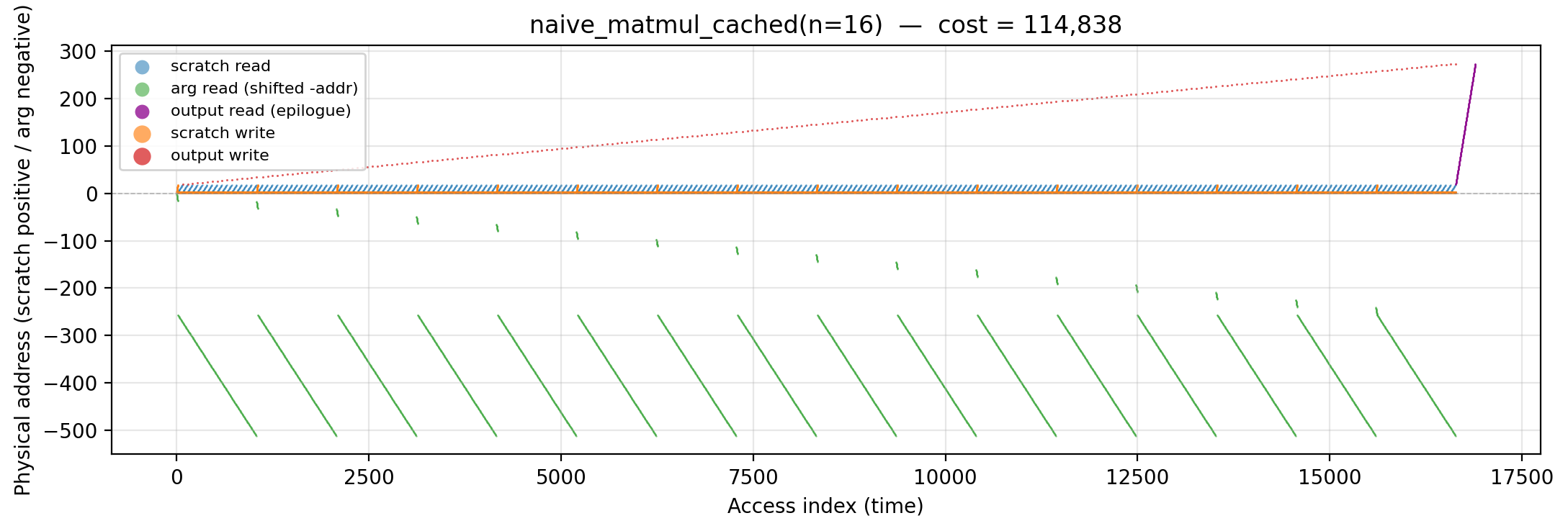
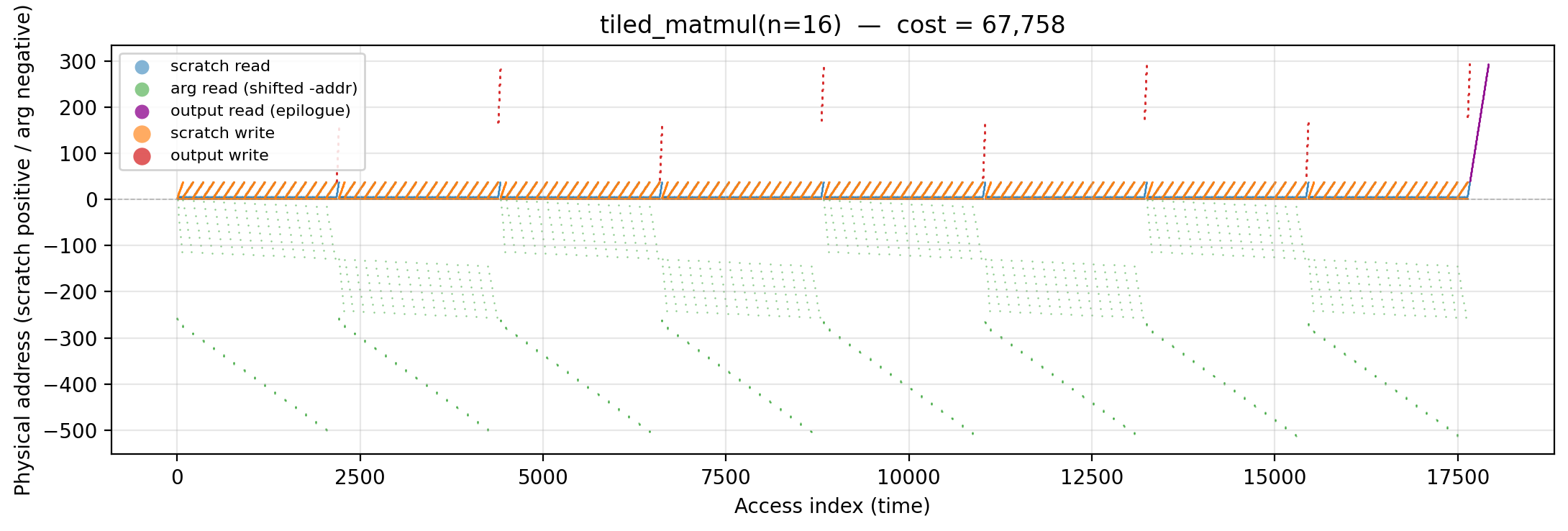
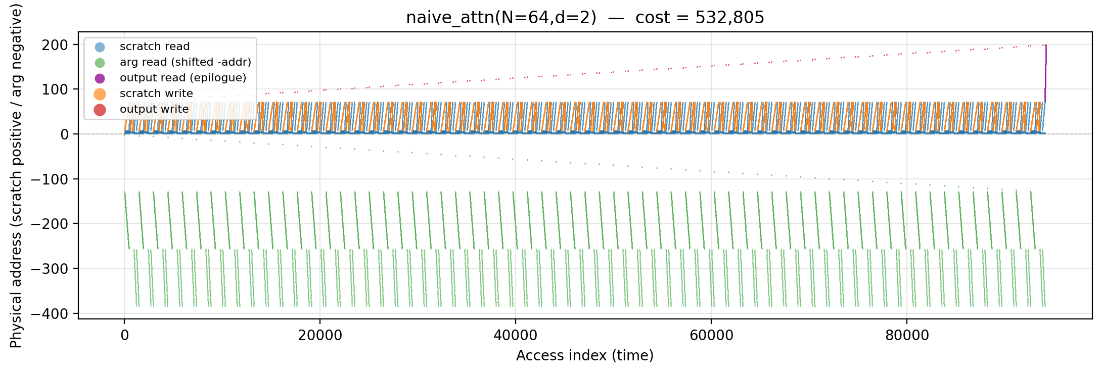
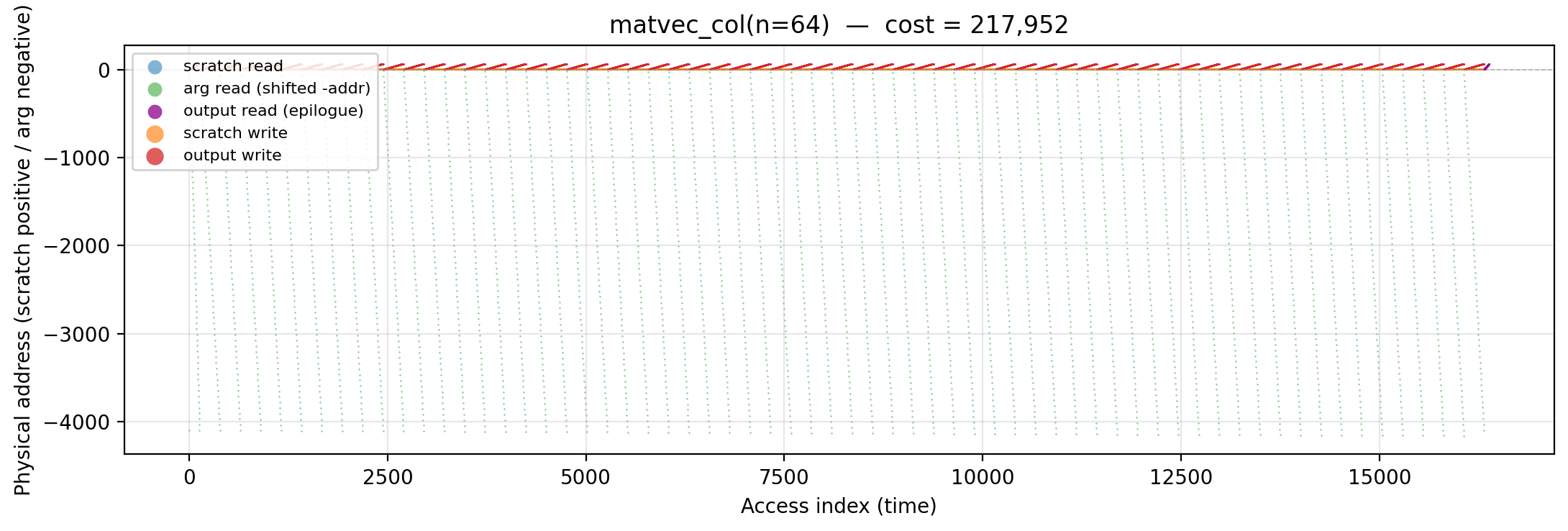
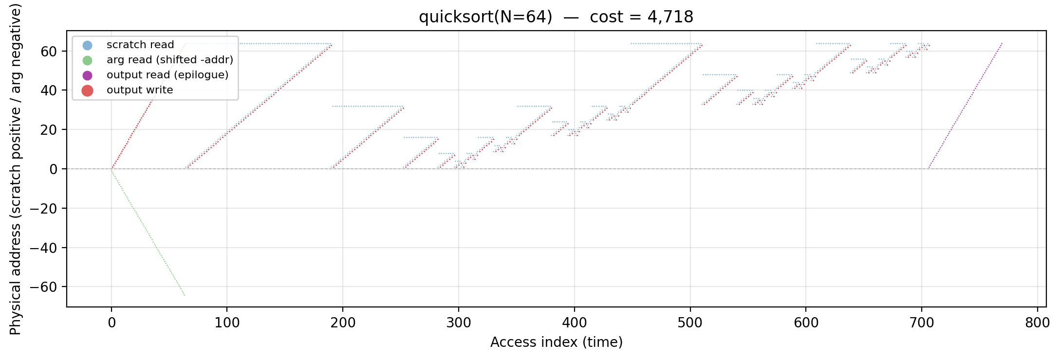
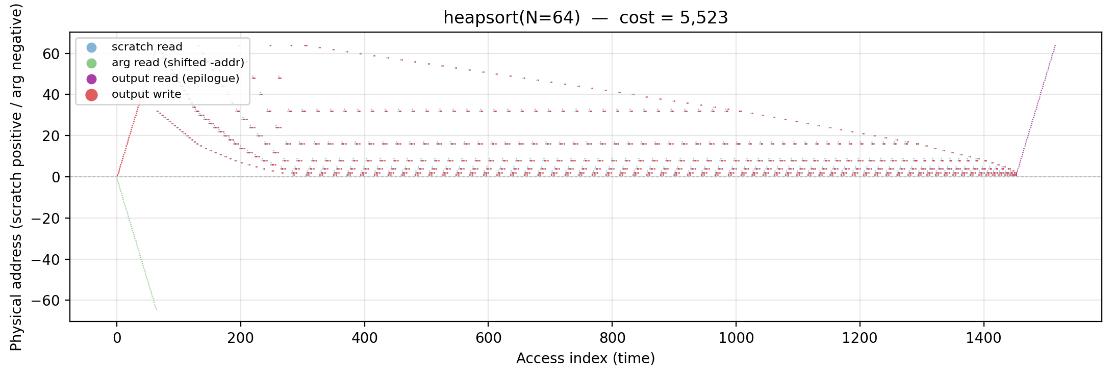
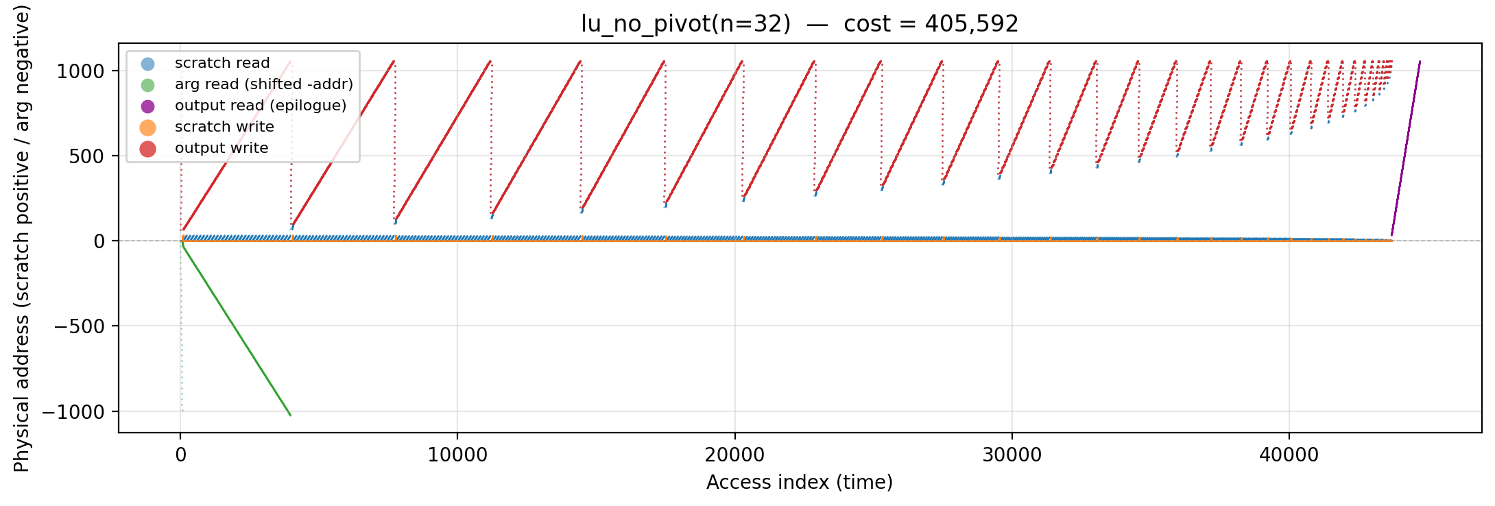
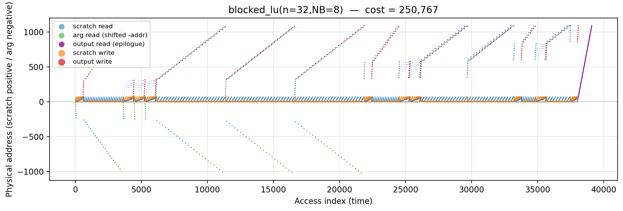
<slug>.png |
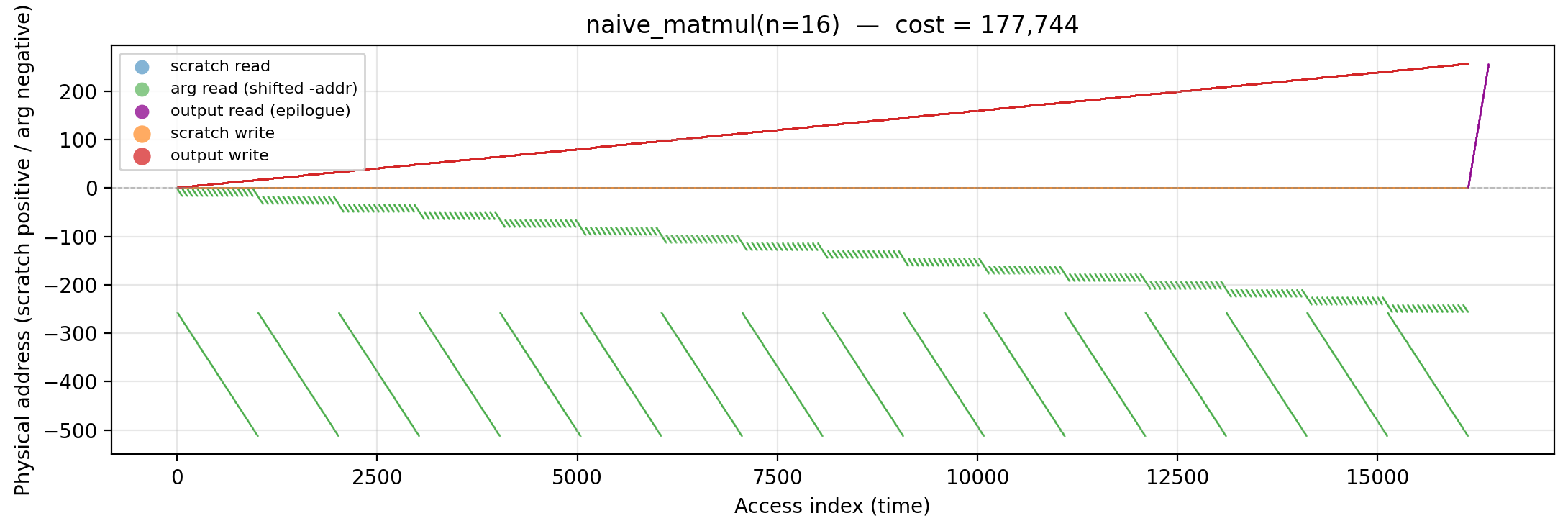
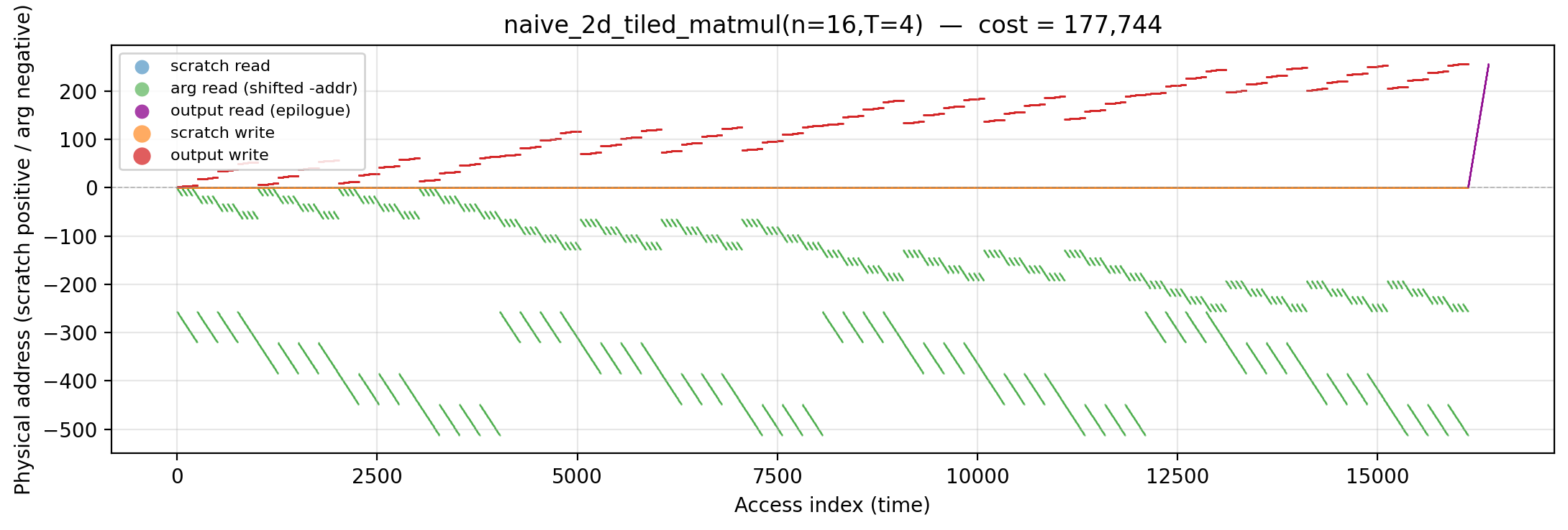
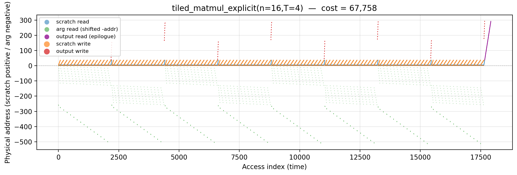
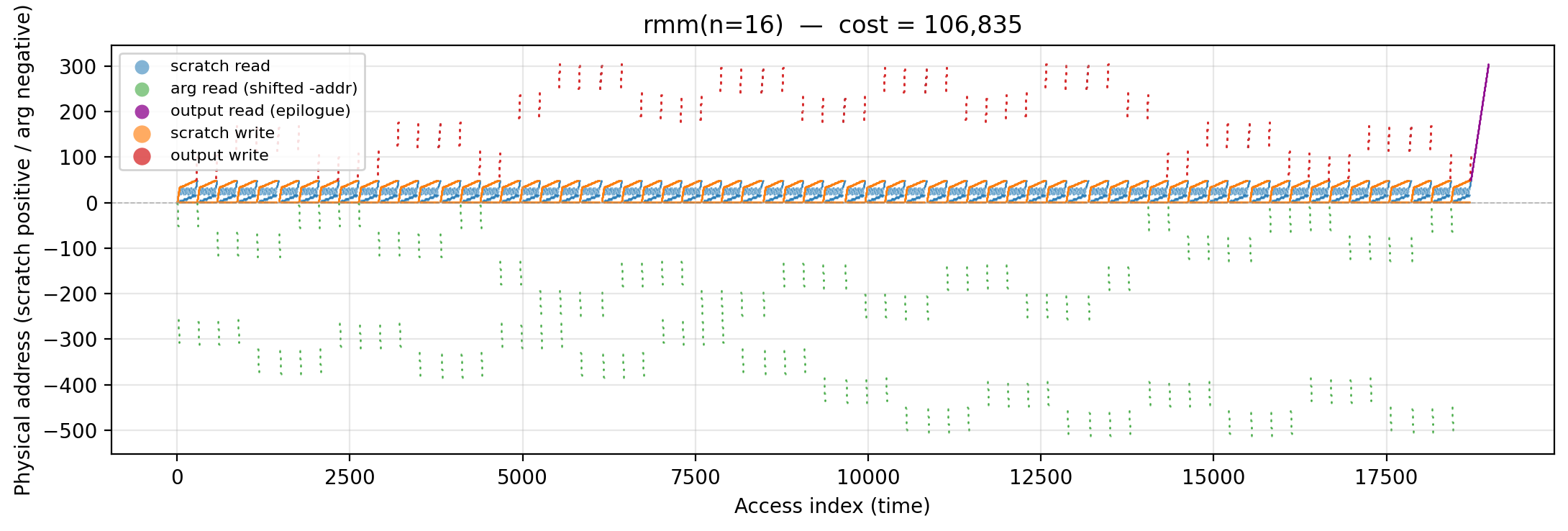
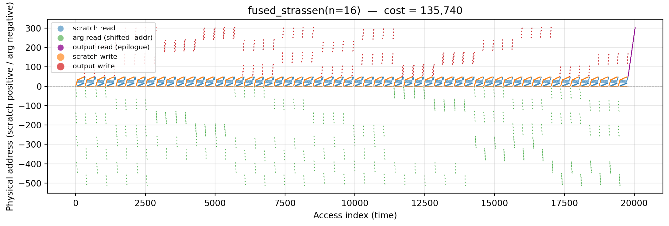
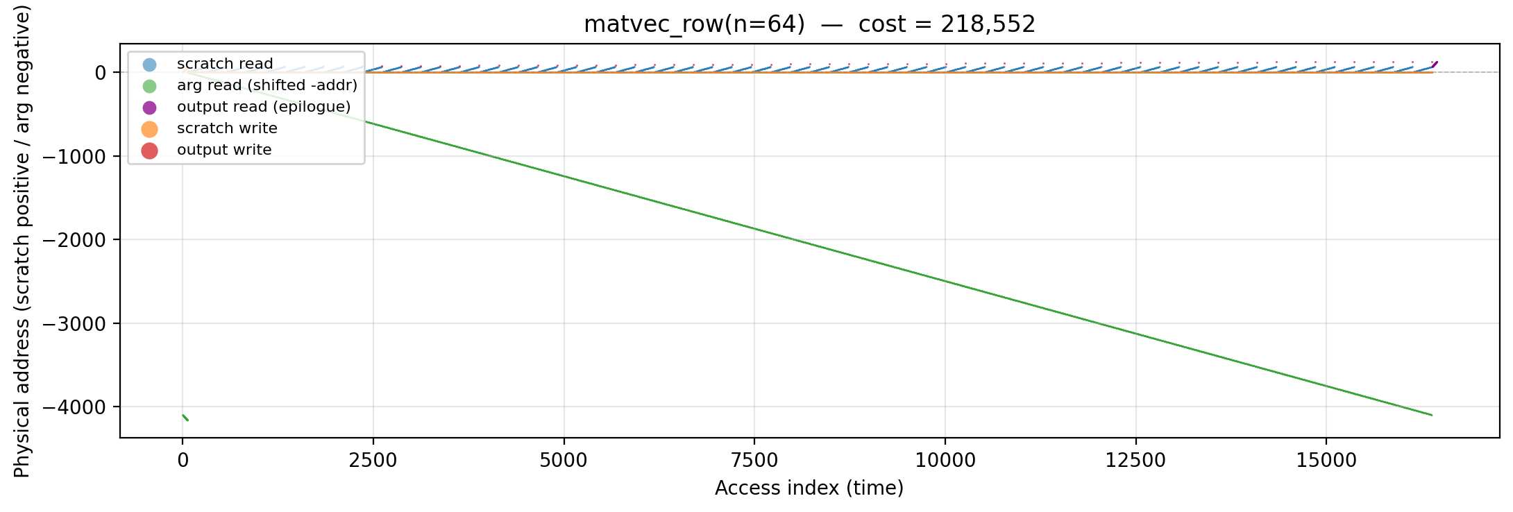
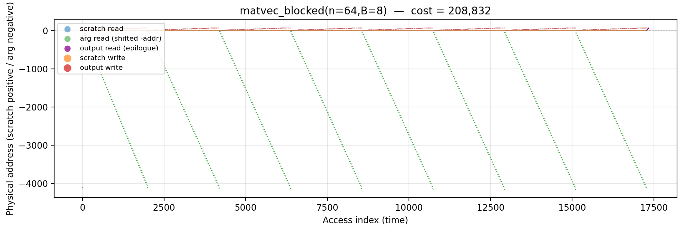
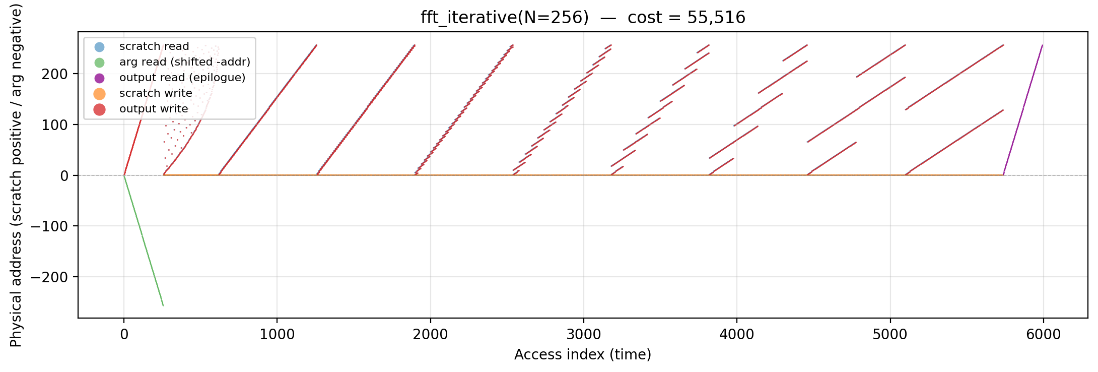
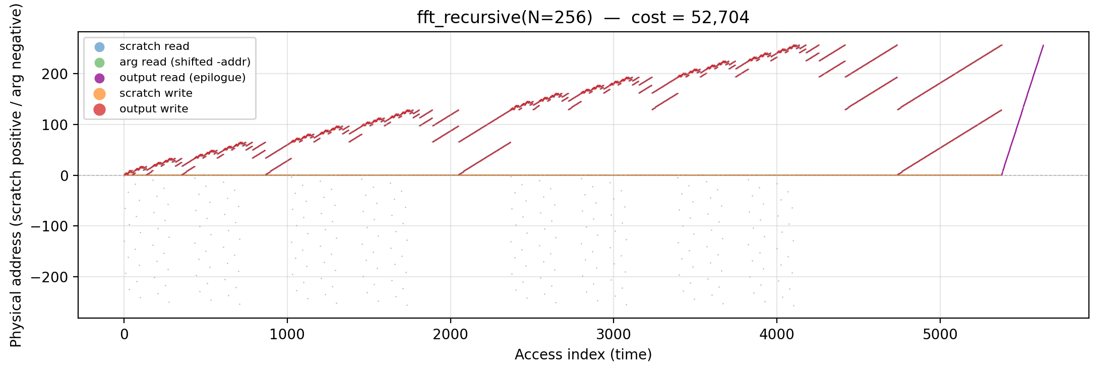
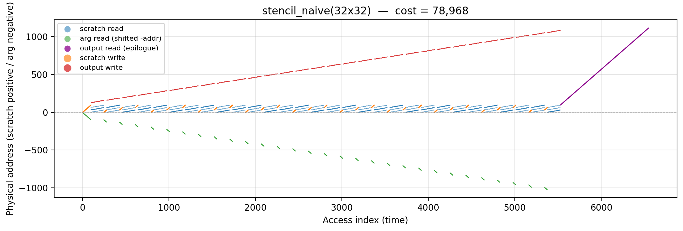
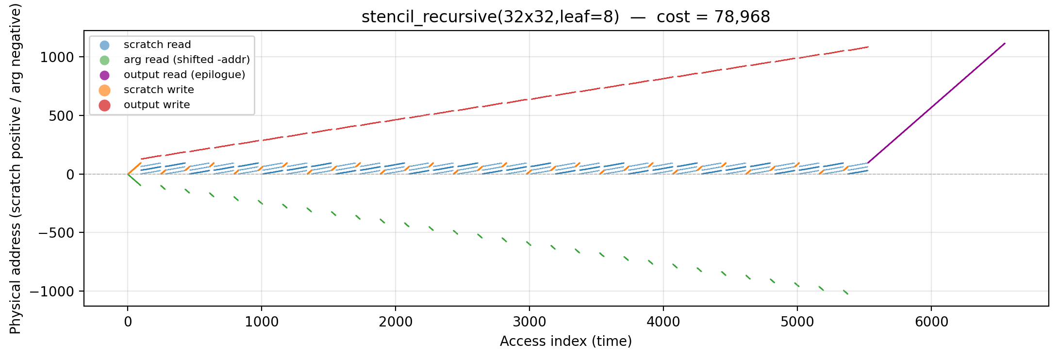
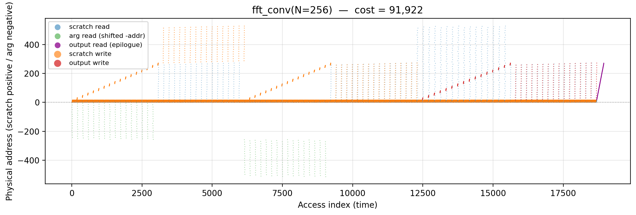
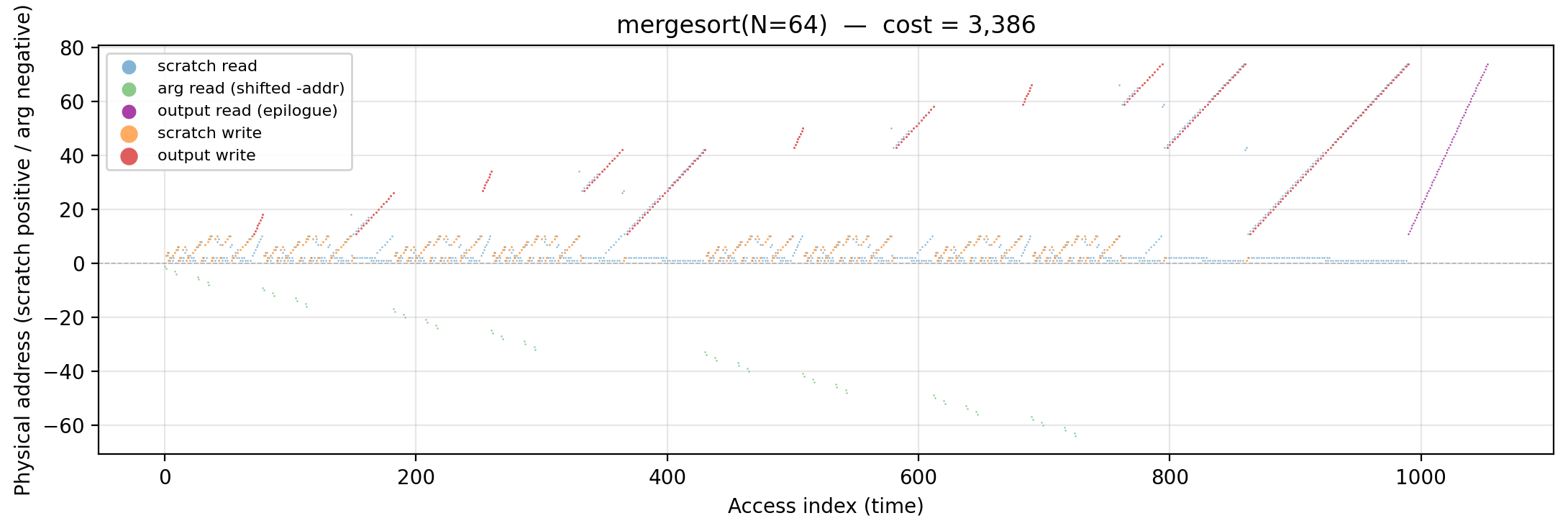
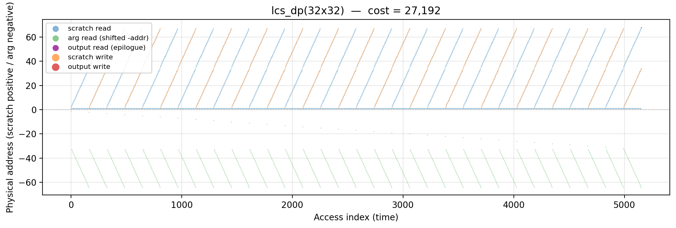
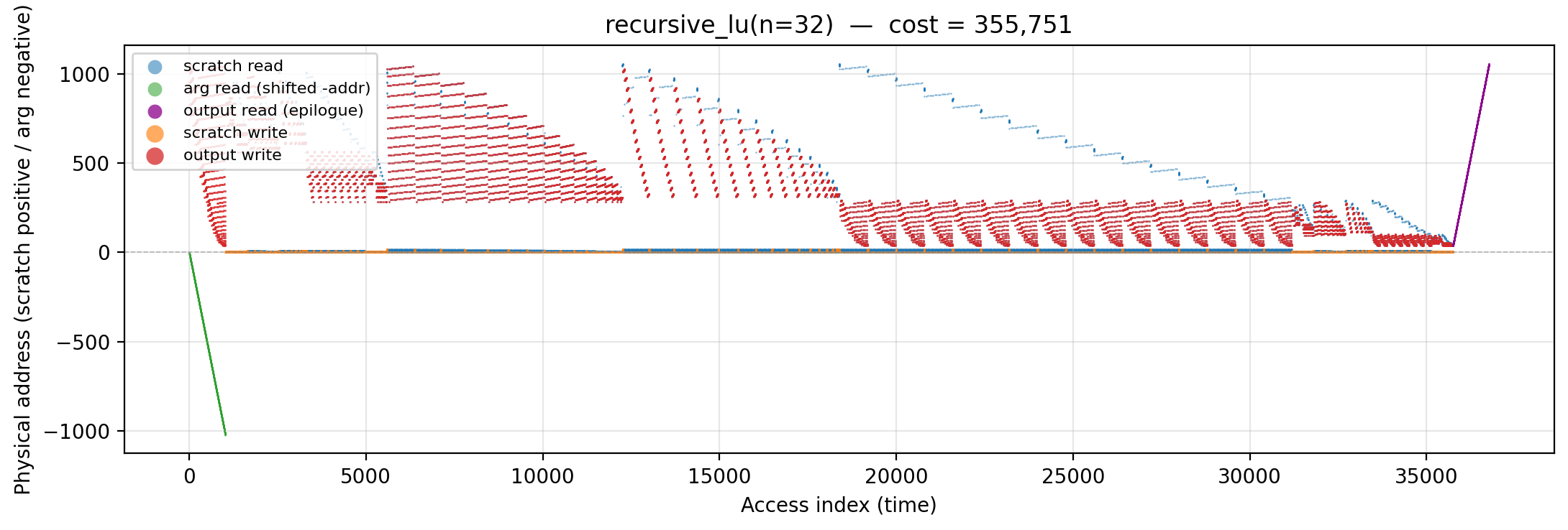
Two-stack scatter of every memory access. Arg-stack reads plot at −addr, scratch reads at +addr. Writes are orange (scratch) / red (output); the dark-magenta band on top is the output epilogue read. |
— |
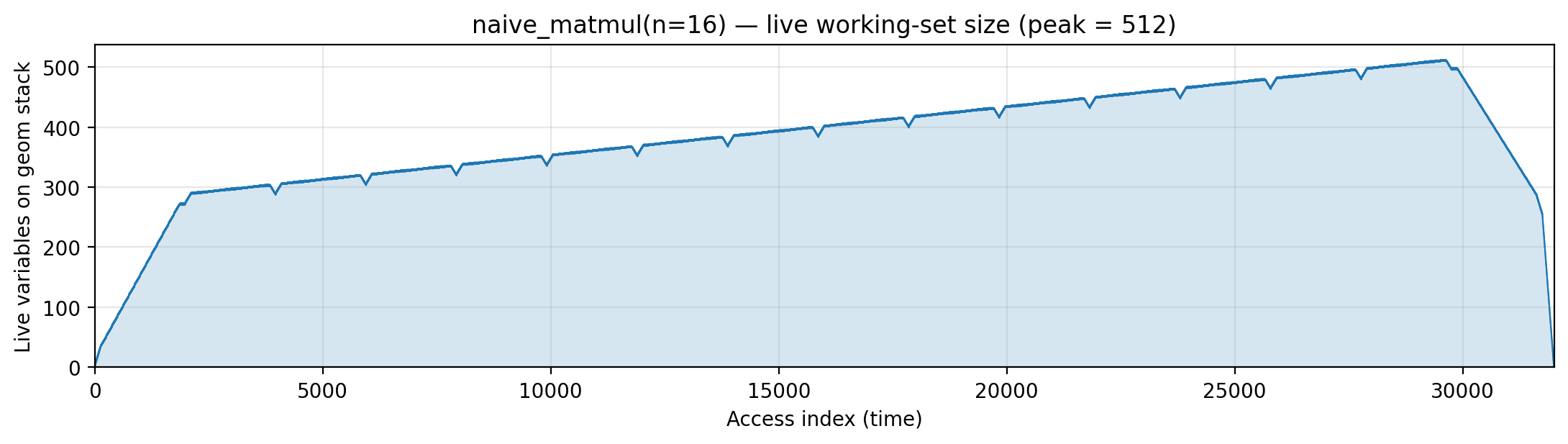
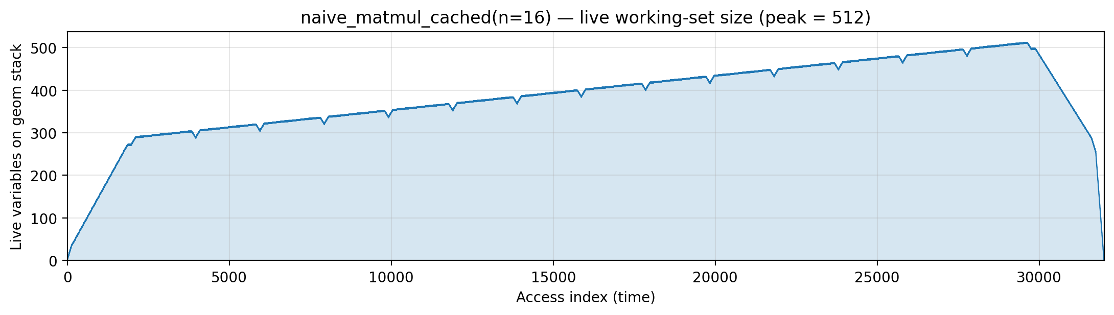
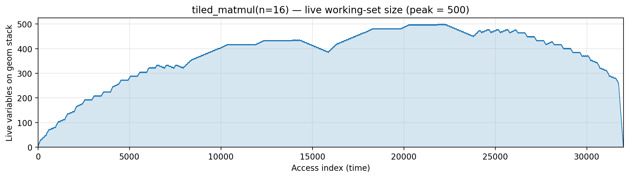
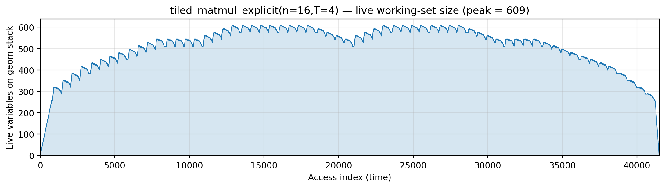
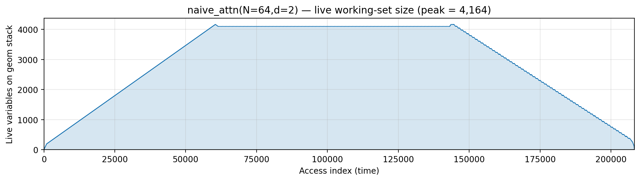
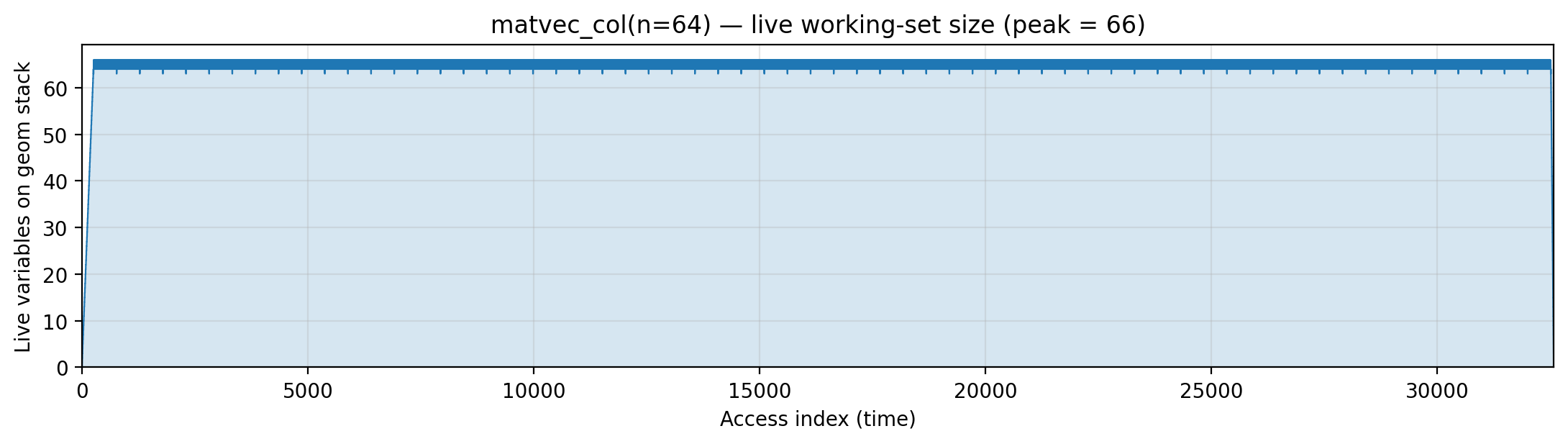
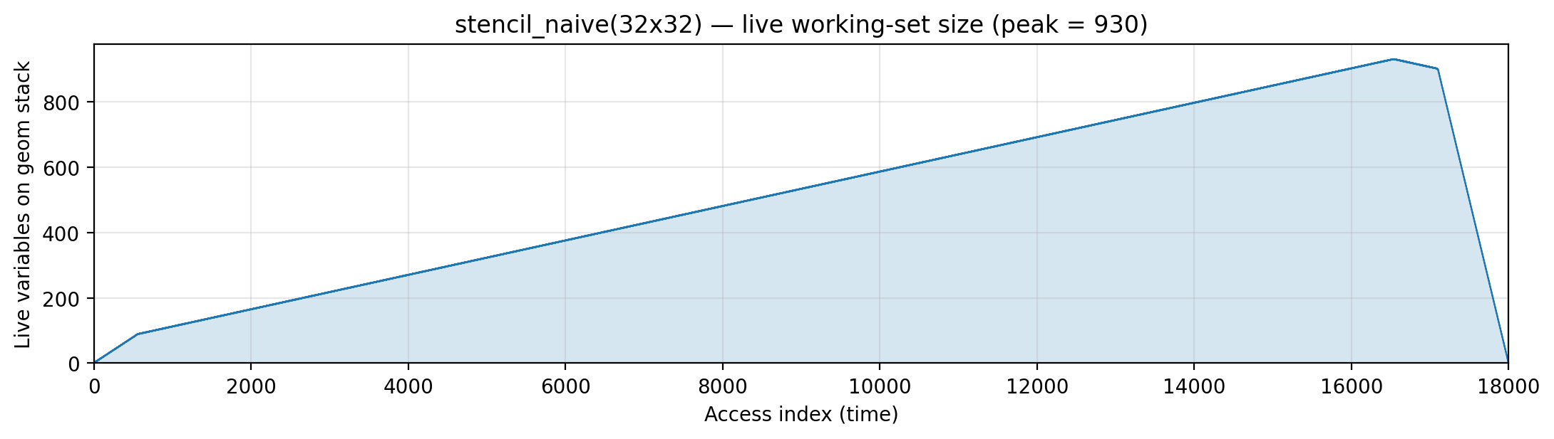
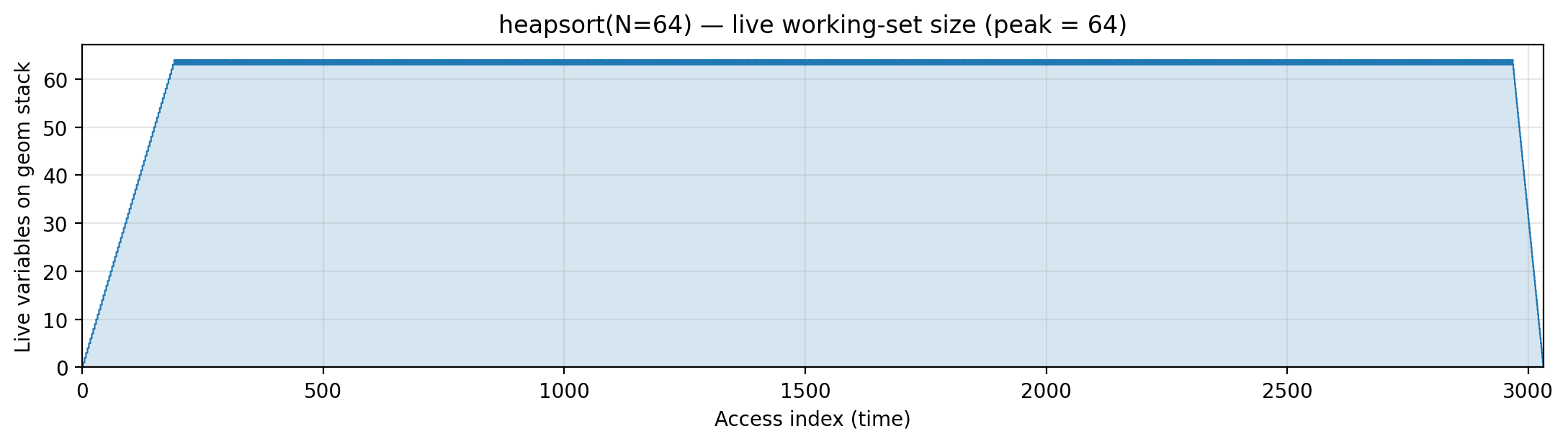
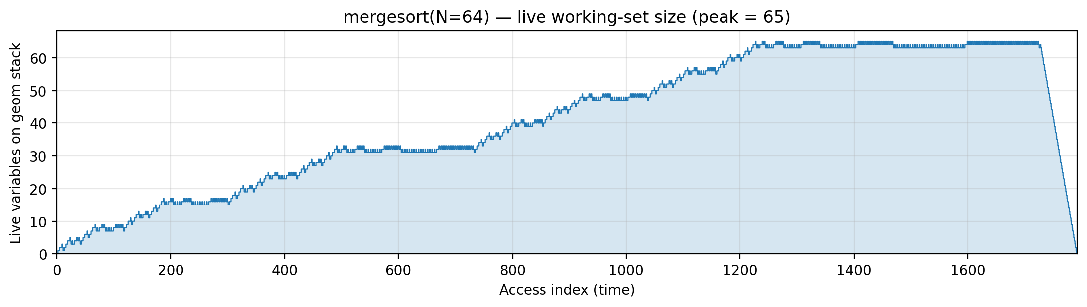
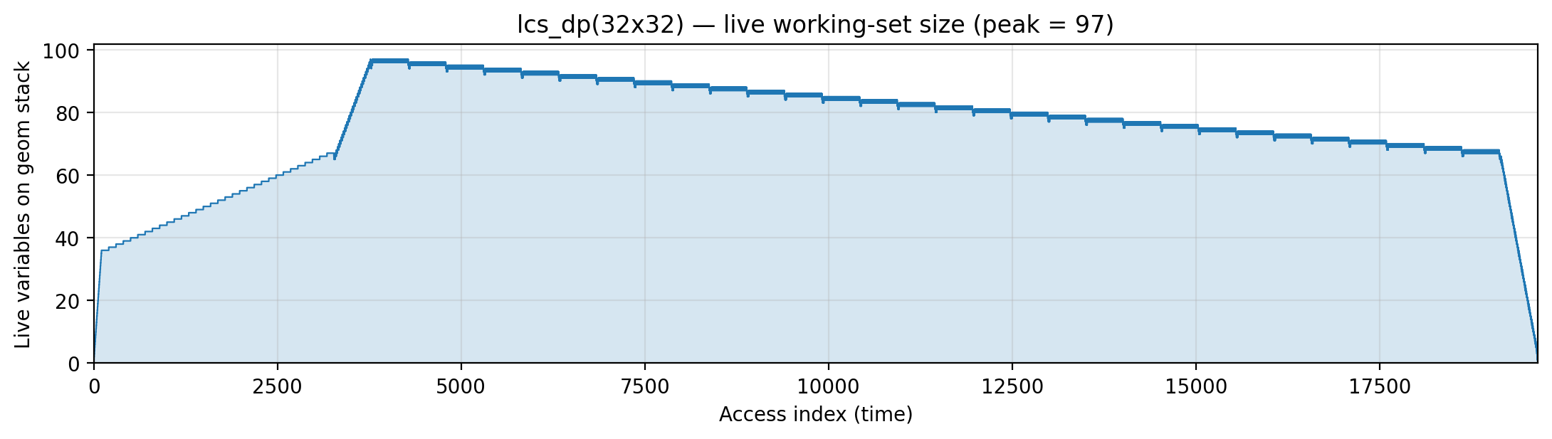
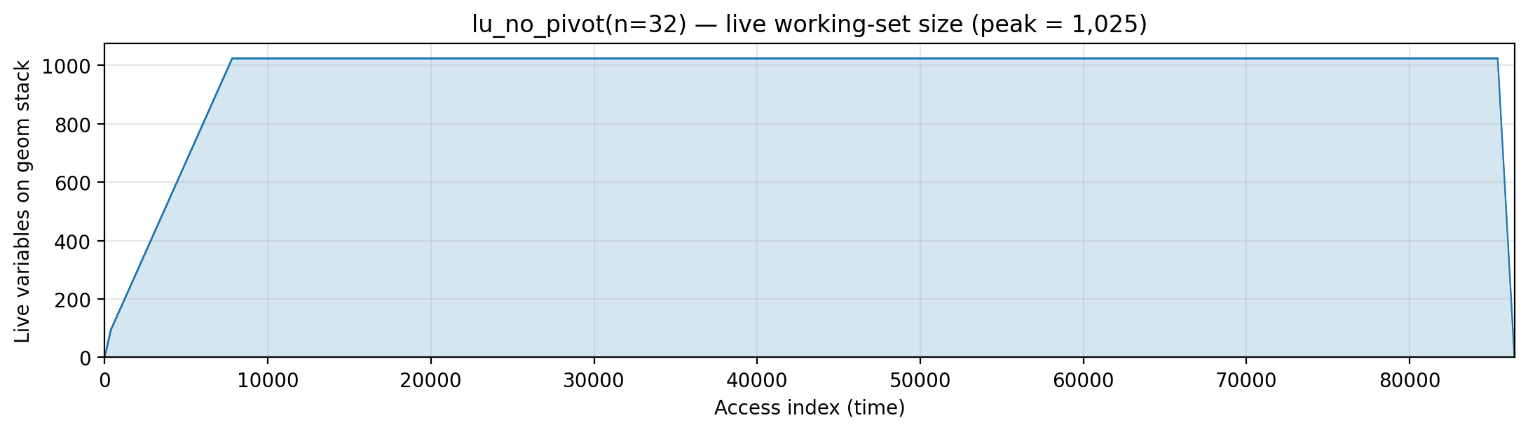
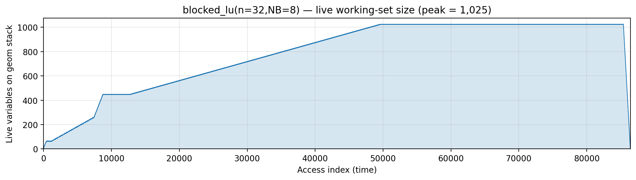
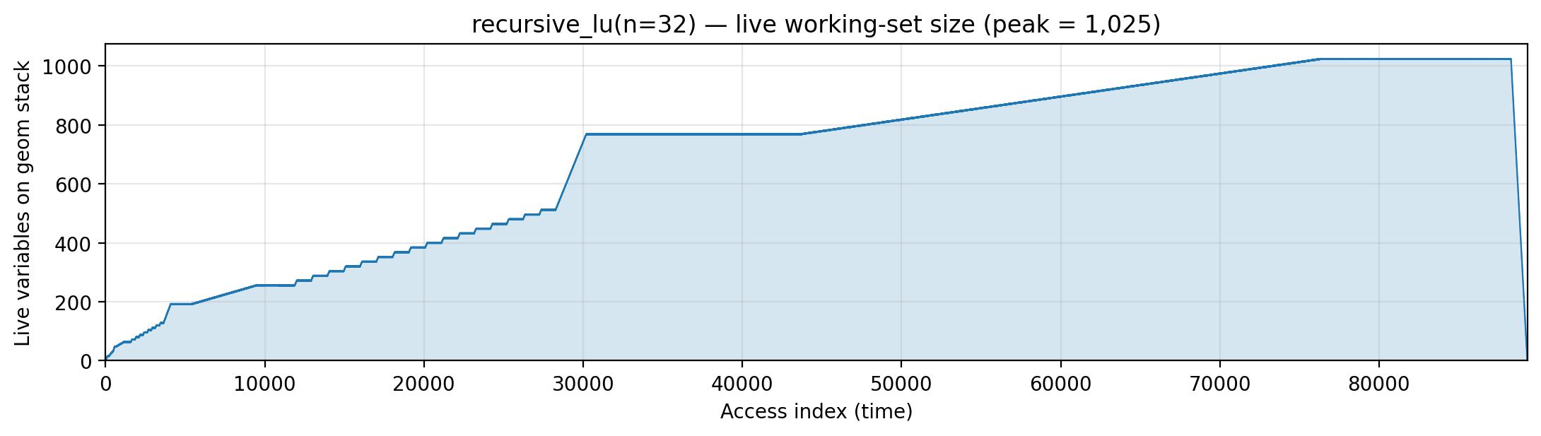
<slug>_liveset.png |
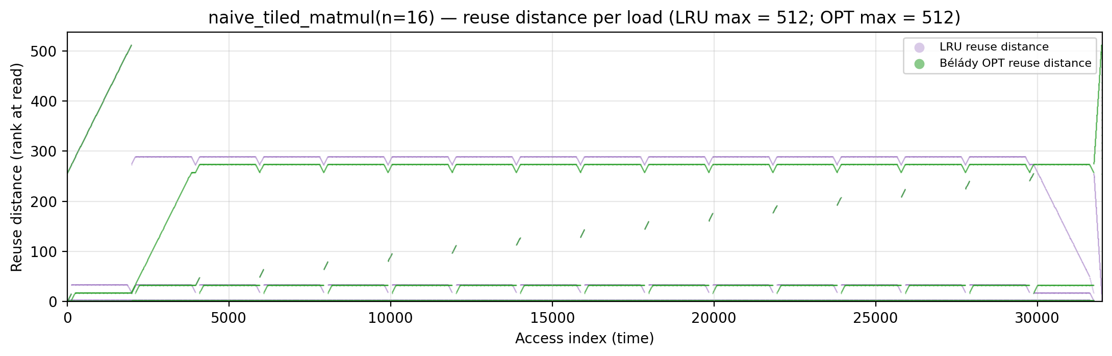
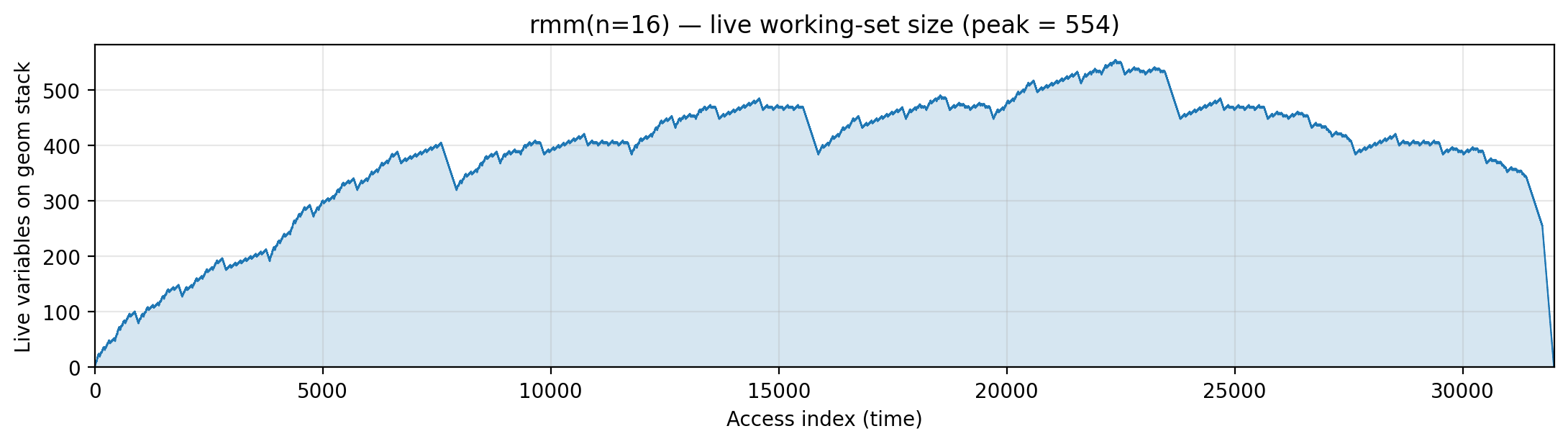
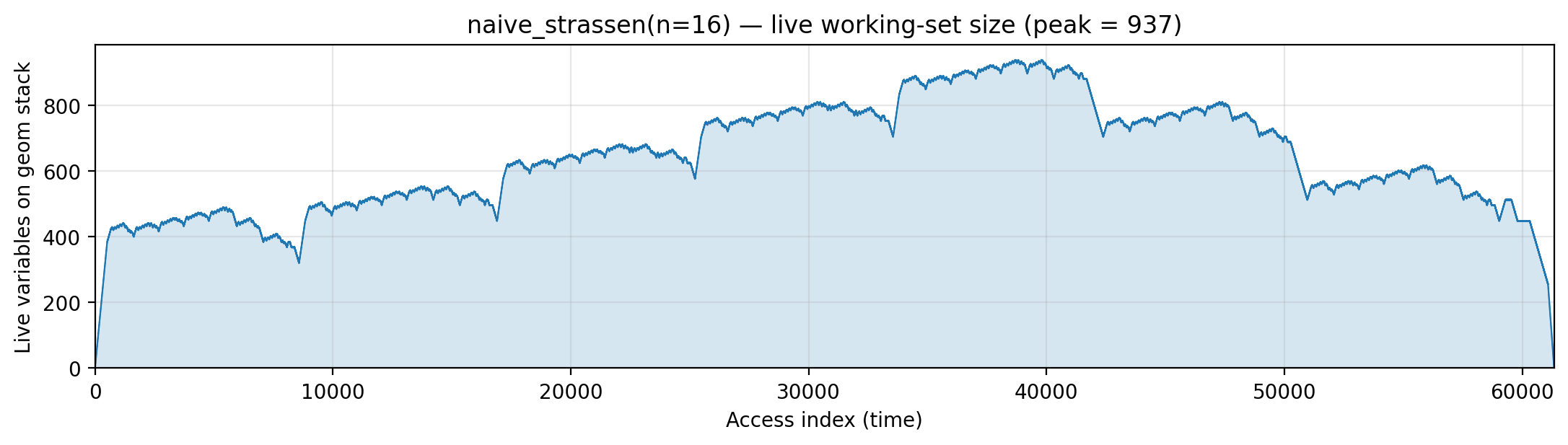
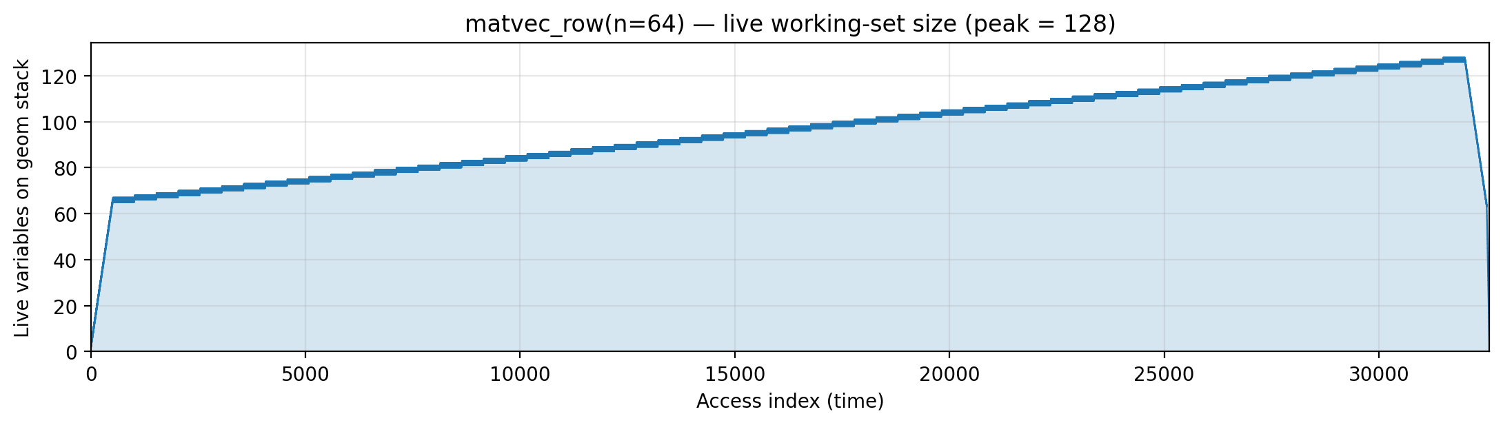
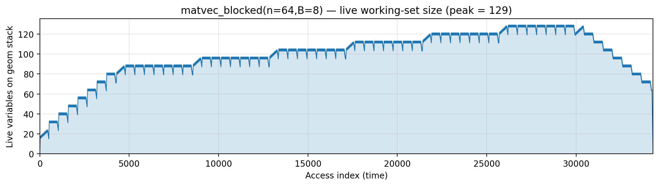
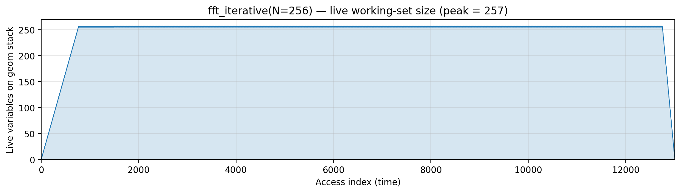
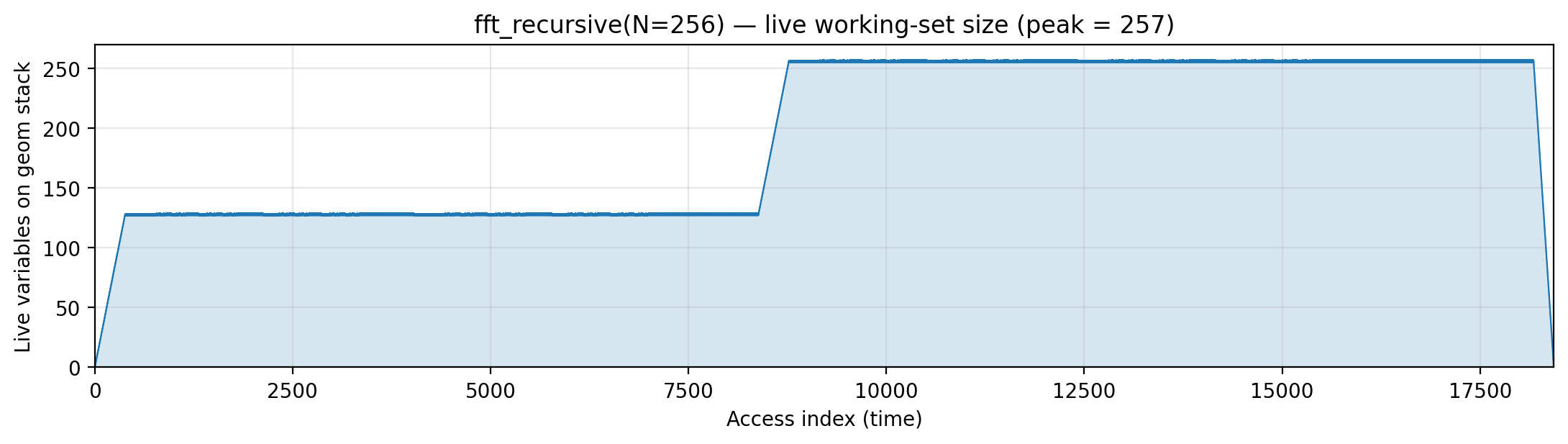
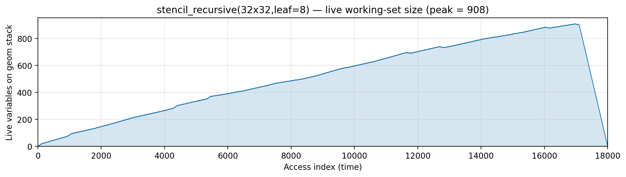
Live working-set size over time on the LRU-live geom stack (vars dropped on last load). | — |
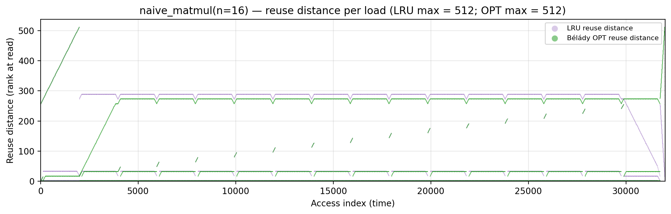
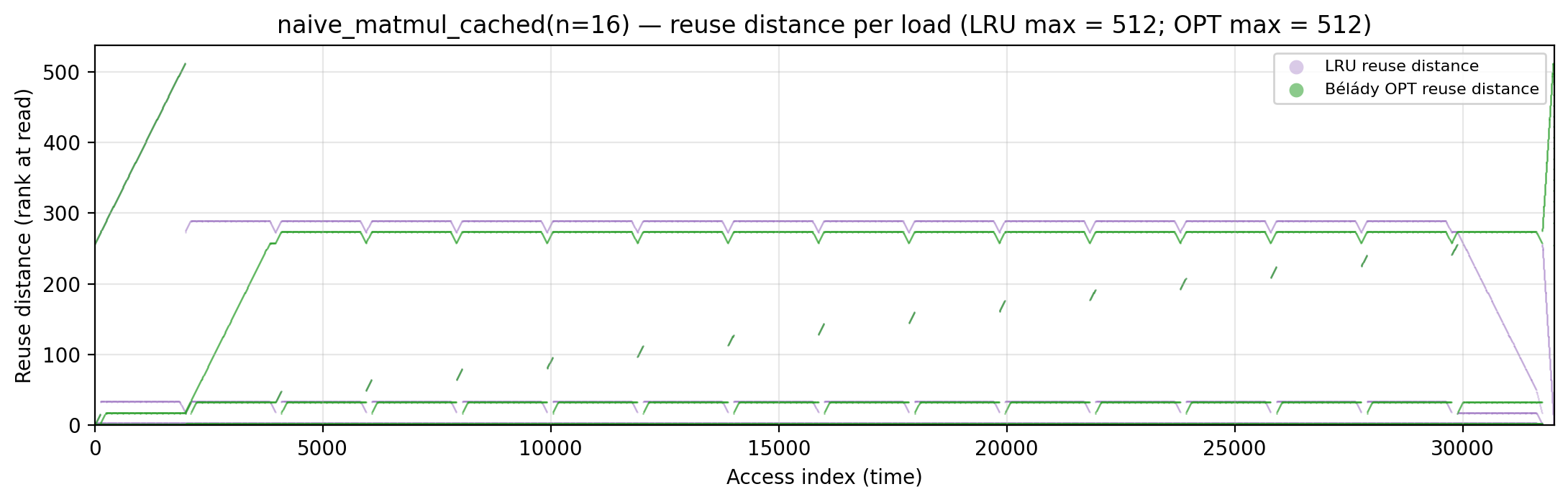
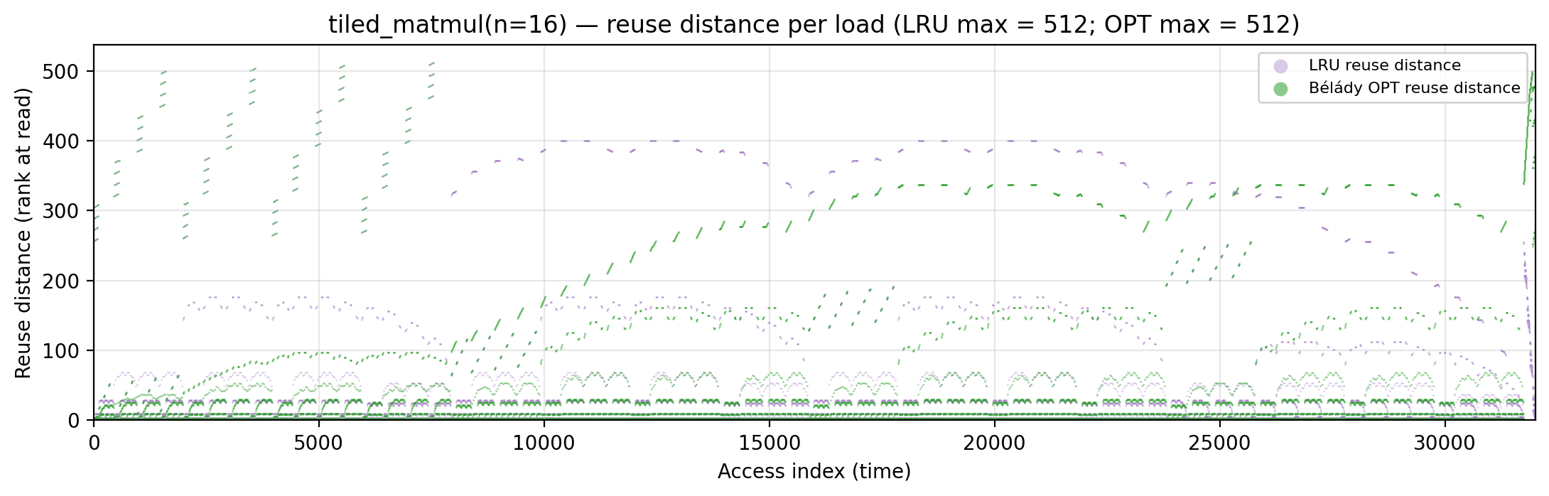
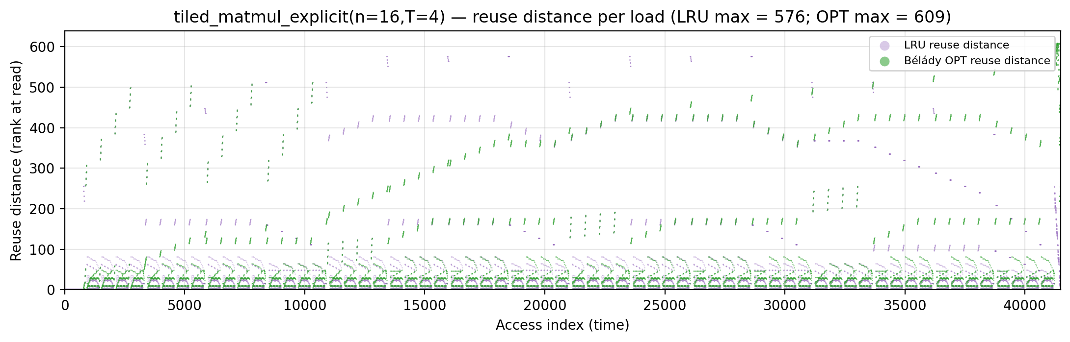
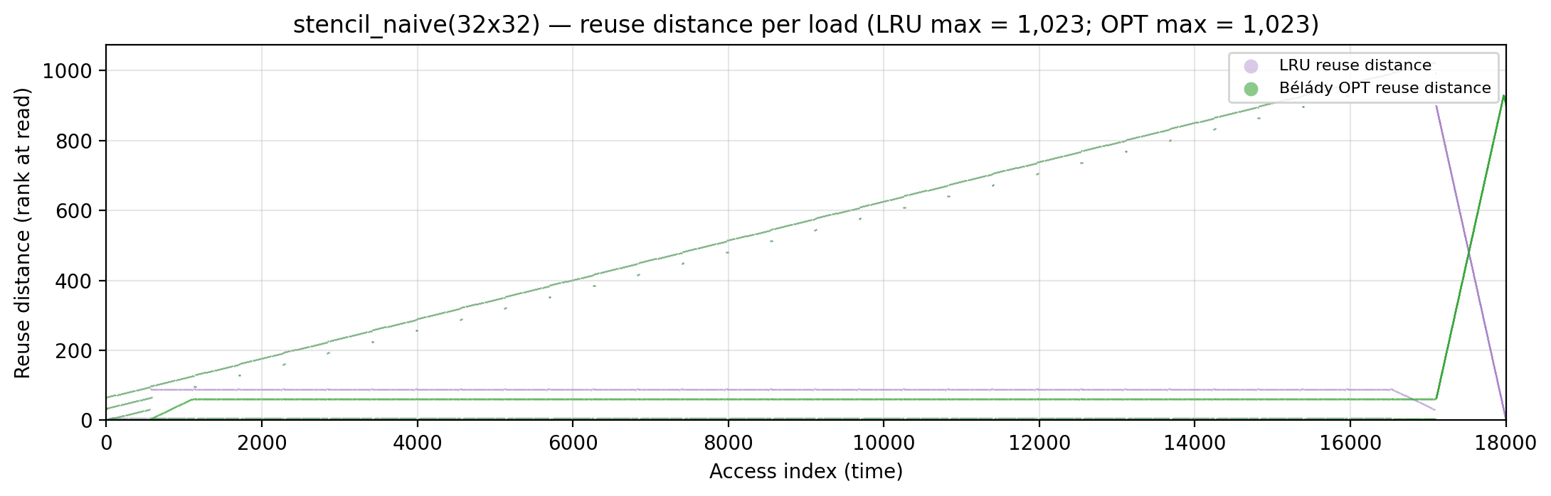
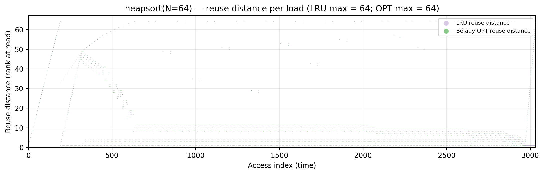
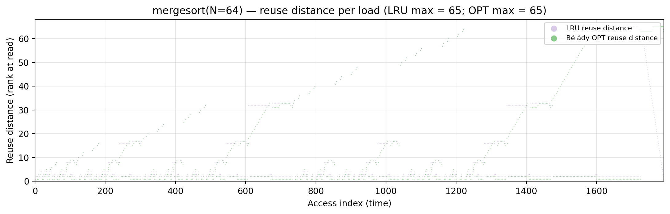
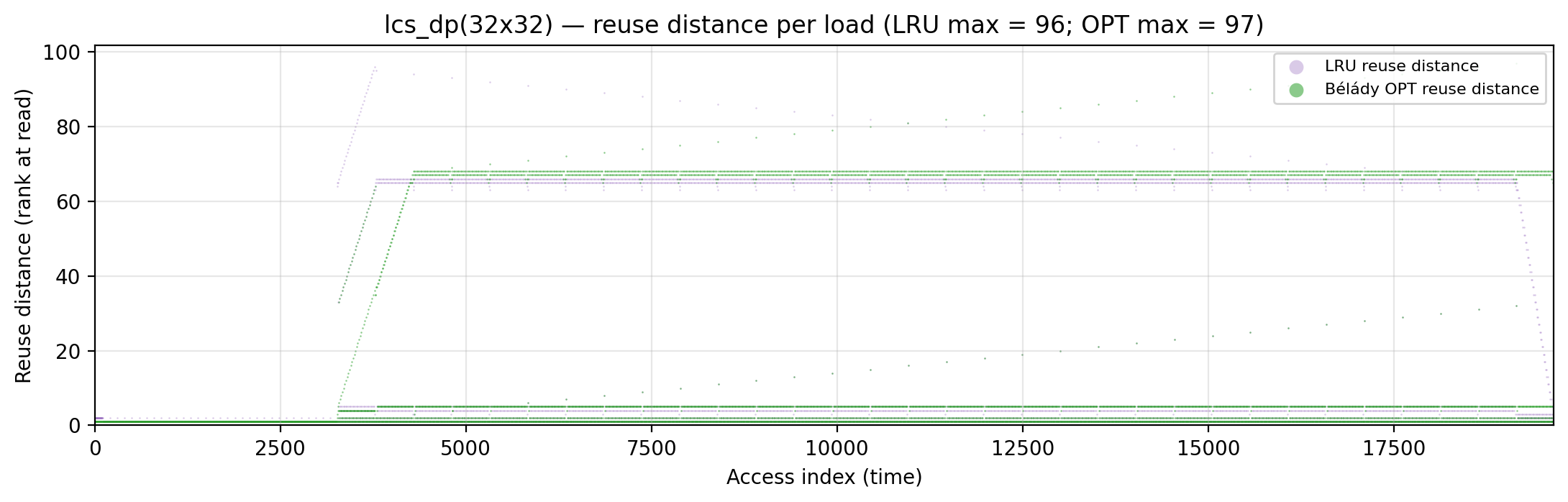
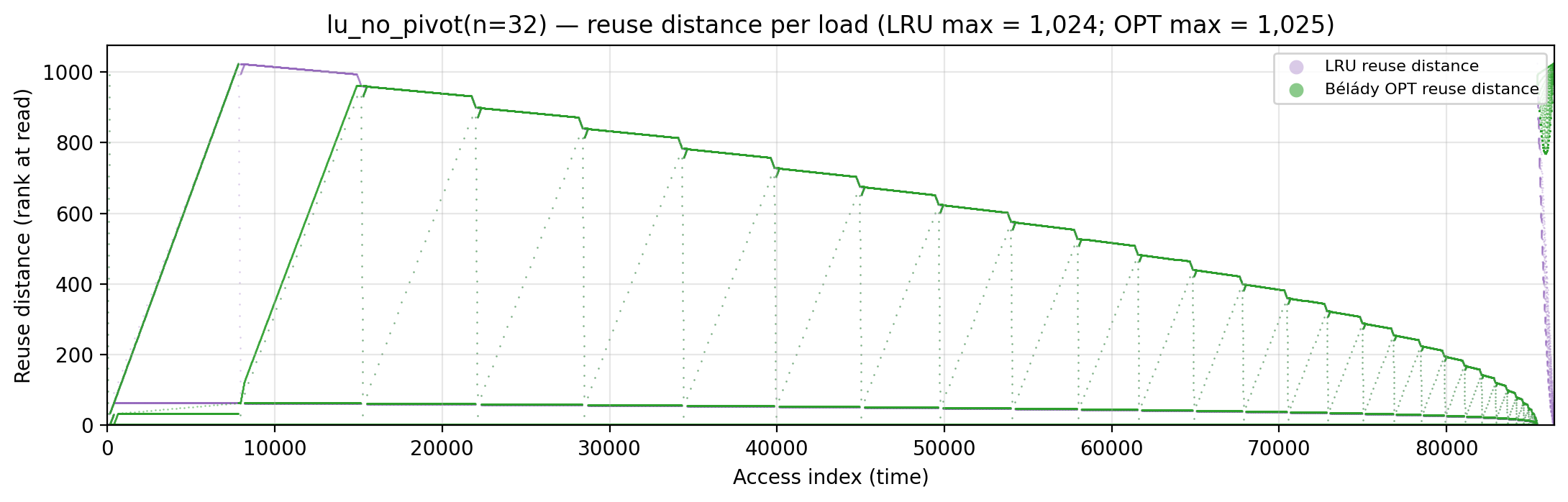
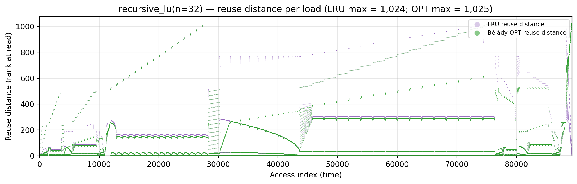
<slug>_reuse_distance.png |
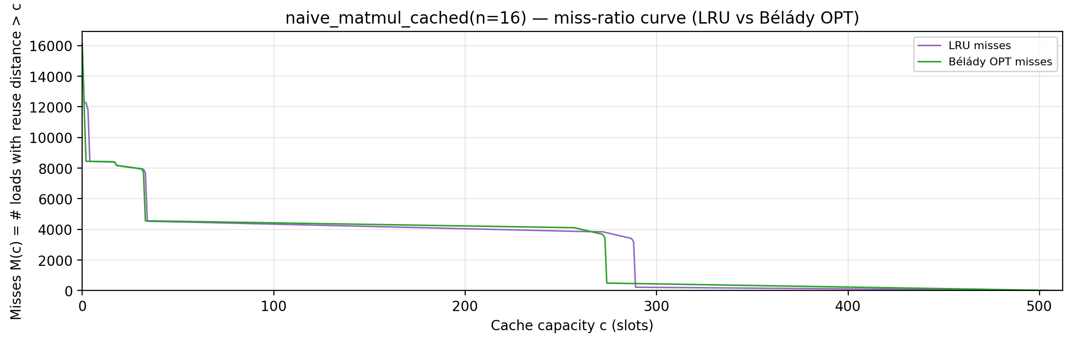
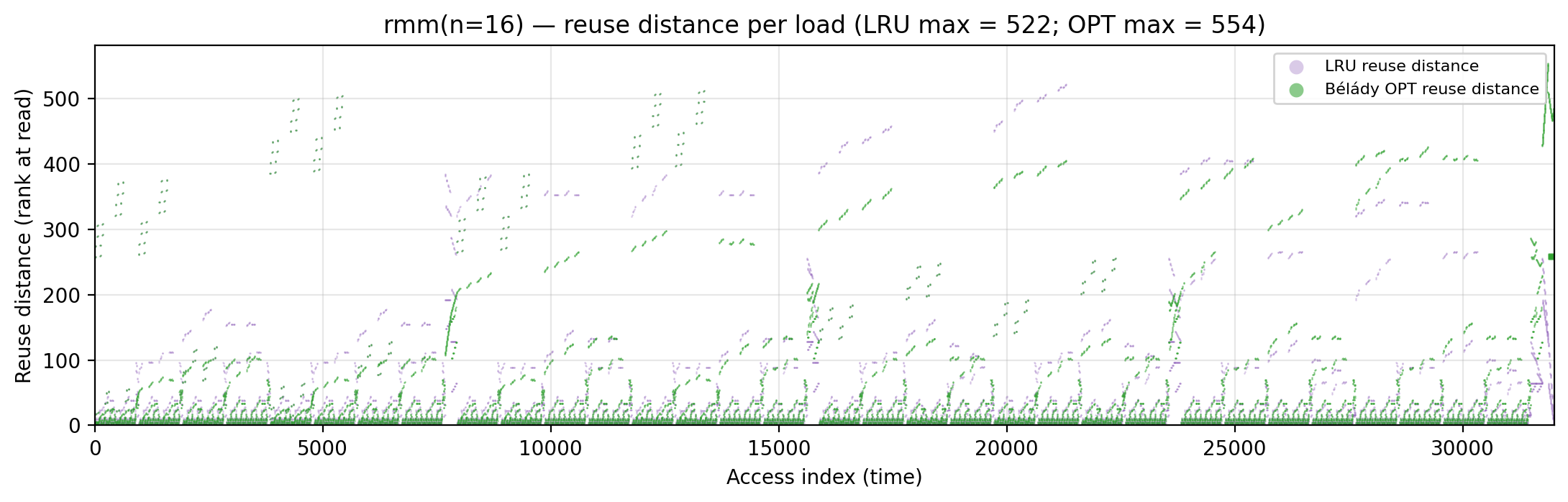
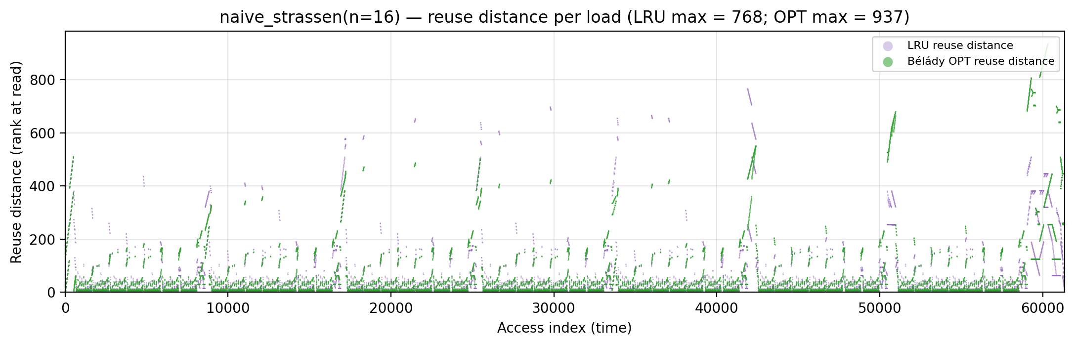
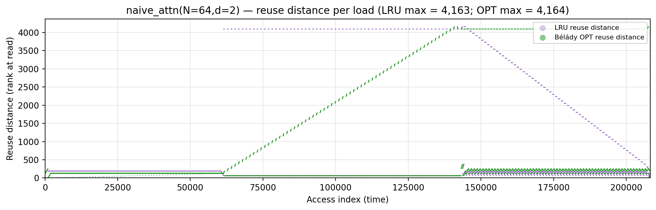
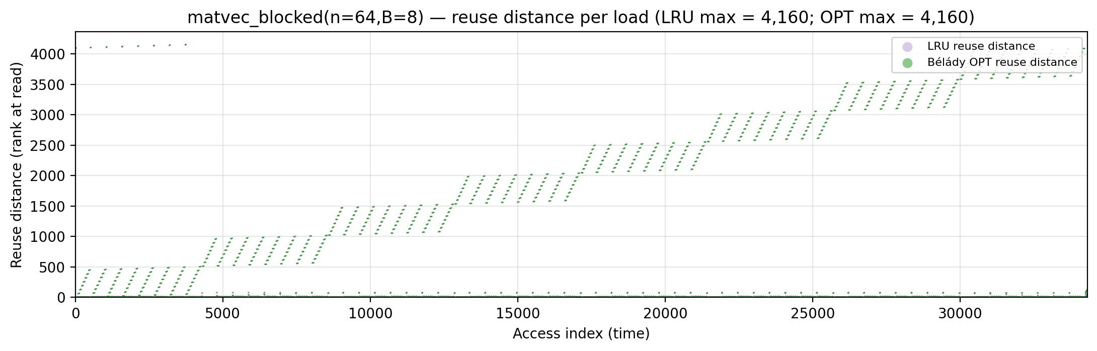
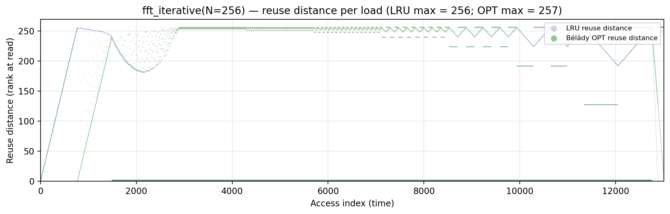
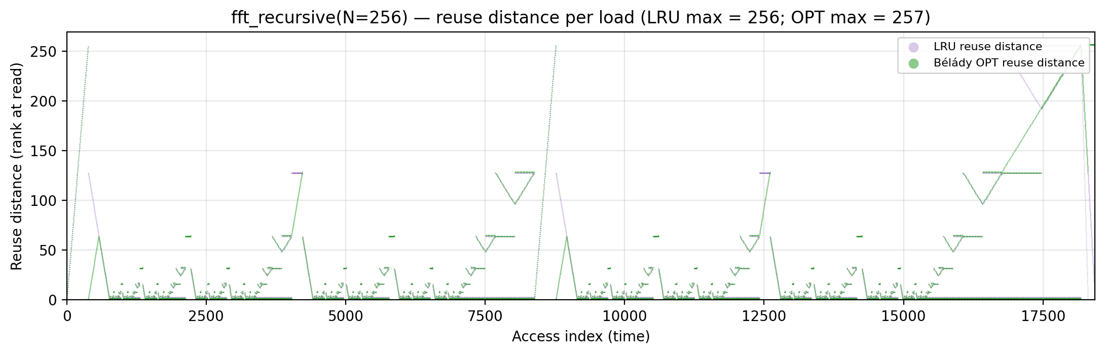
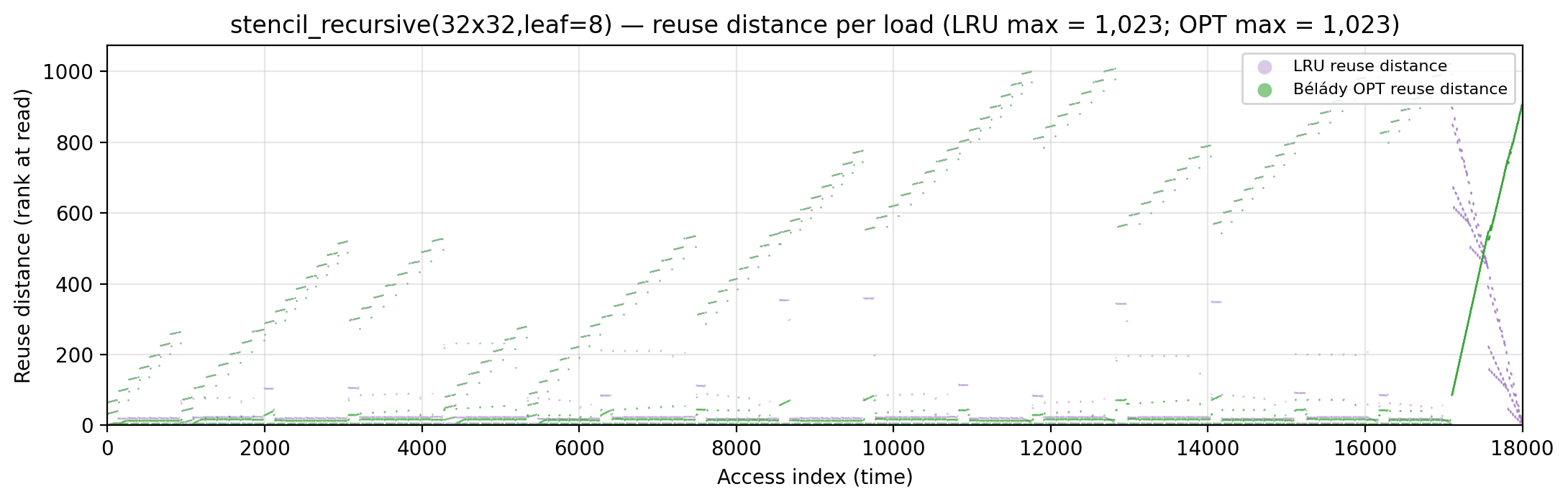
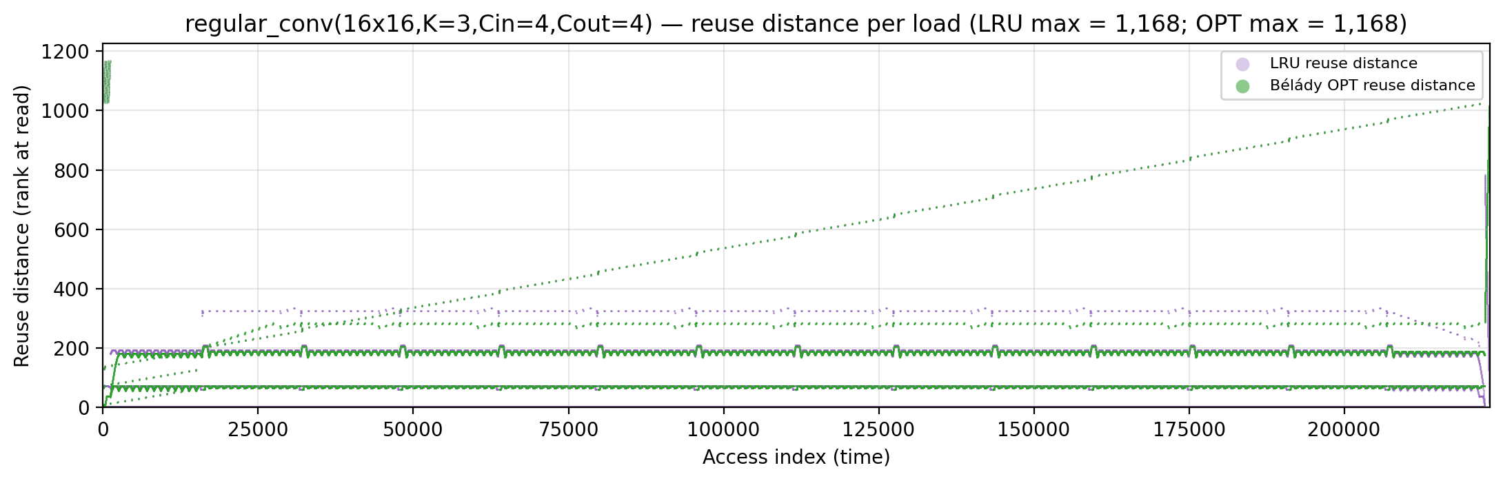
LRU and Bélády OPT reuse distance per load on shared axes (purple = LRU; green = OPT). The visible green-below-purple gap is the locality slack Mattson inclusion guarantees an offline oracle would extract. | belady-min-lower-bound.md |
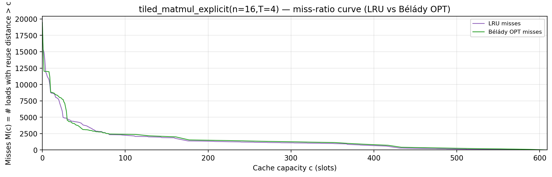
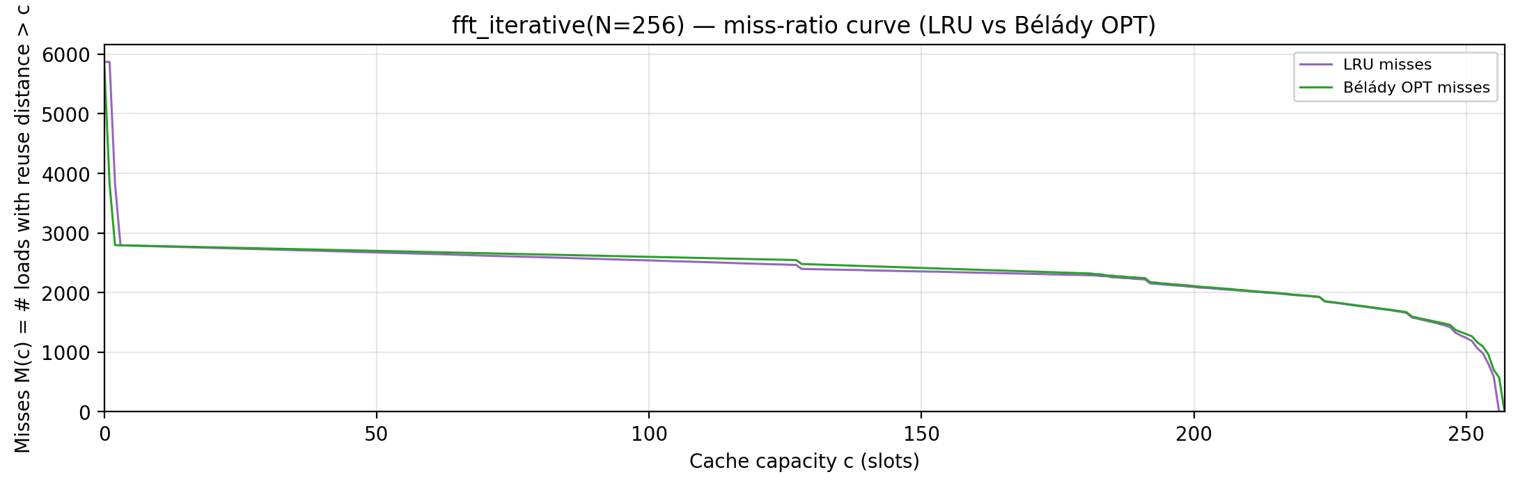
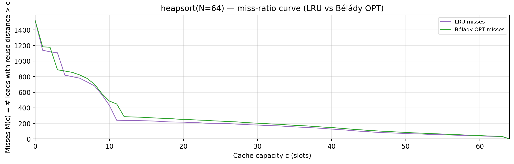
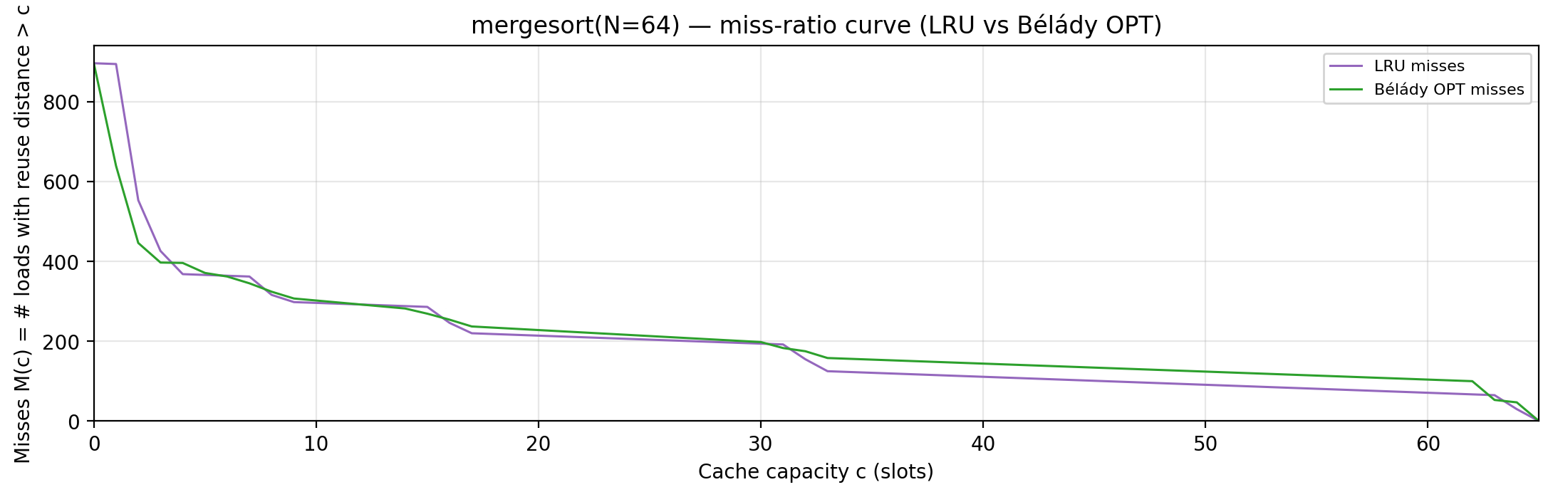
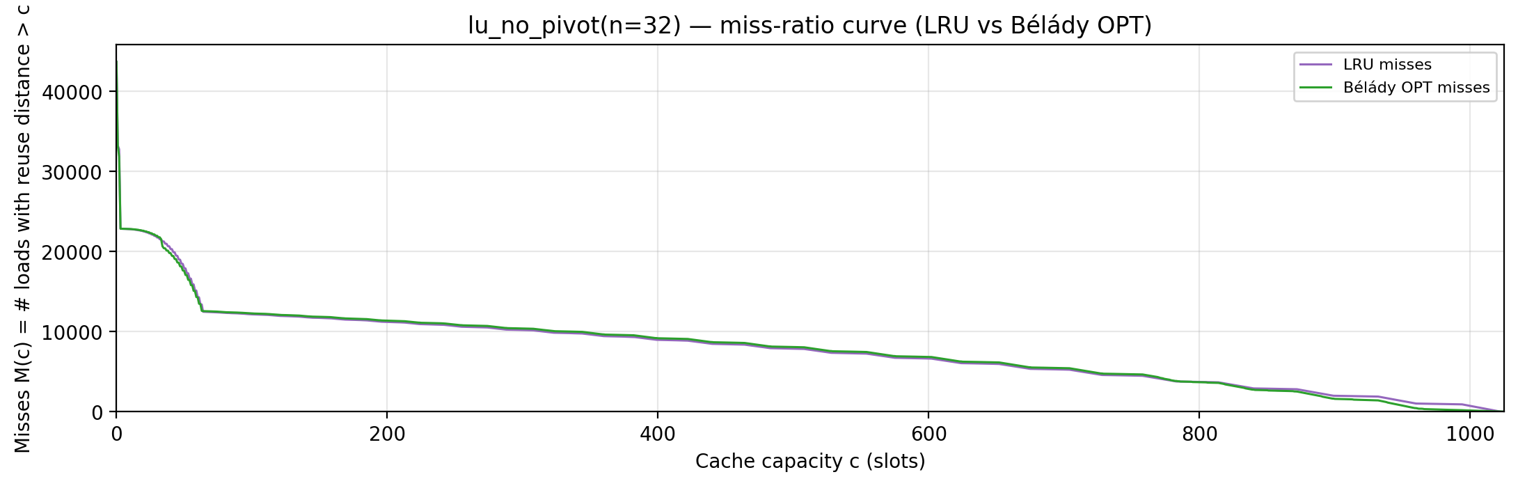
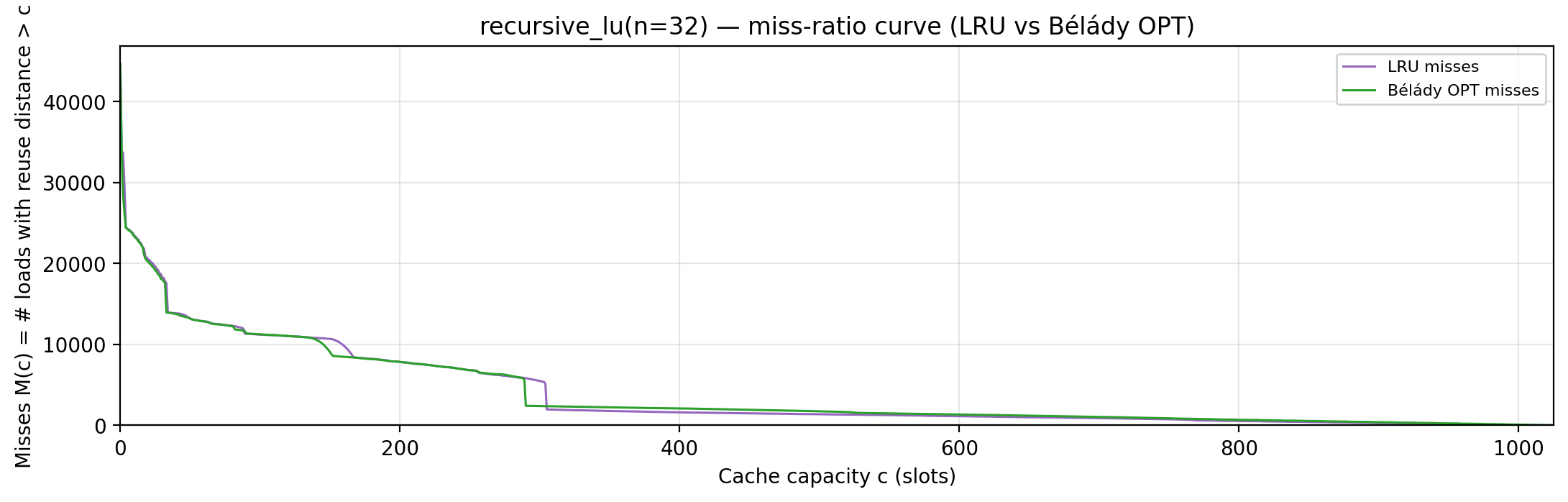
<slug>_mrc.png |
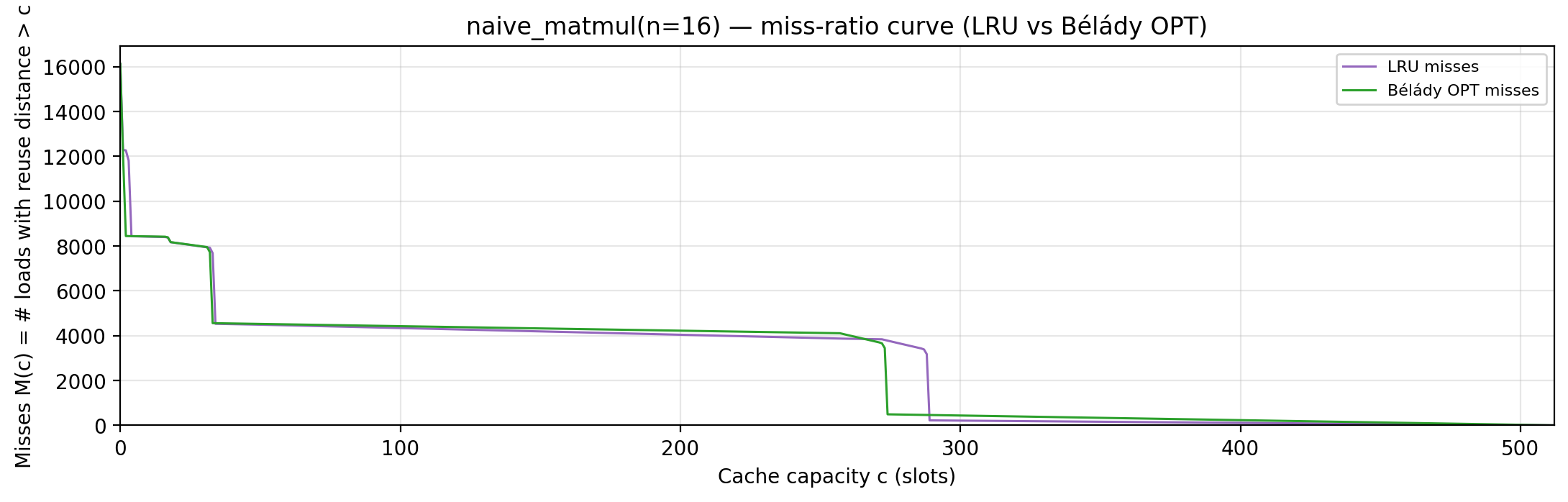
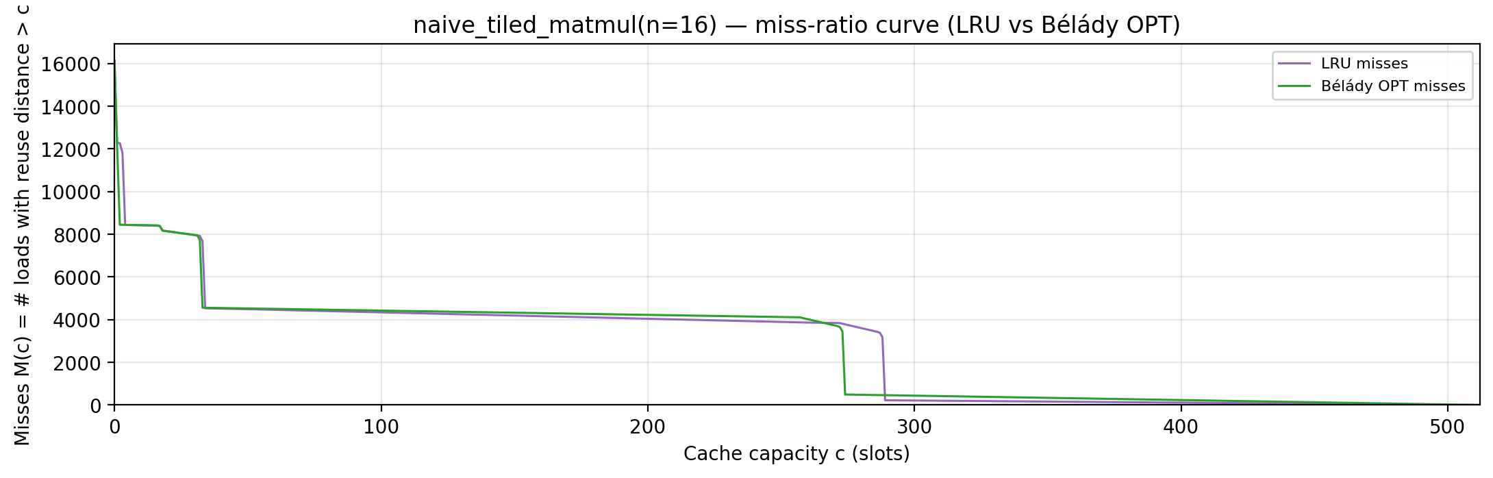
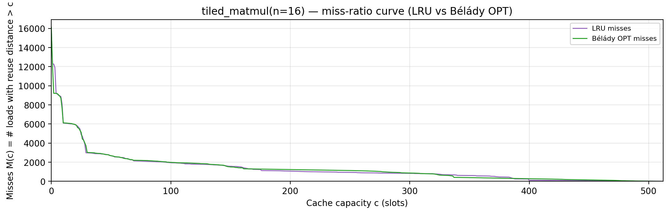
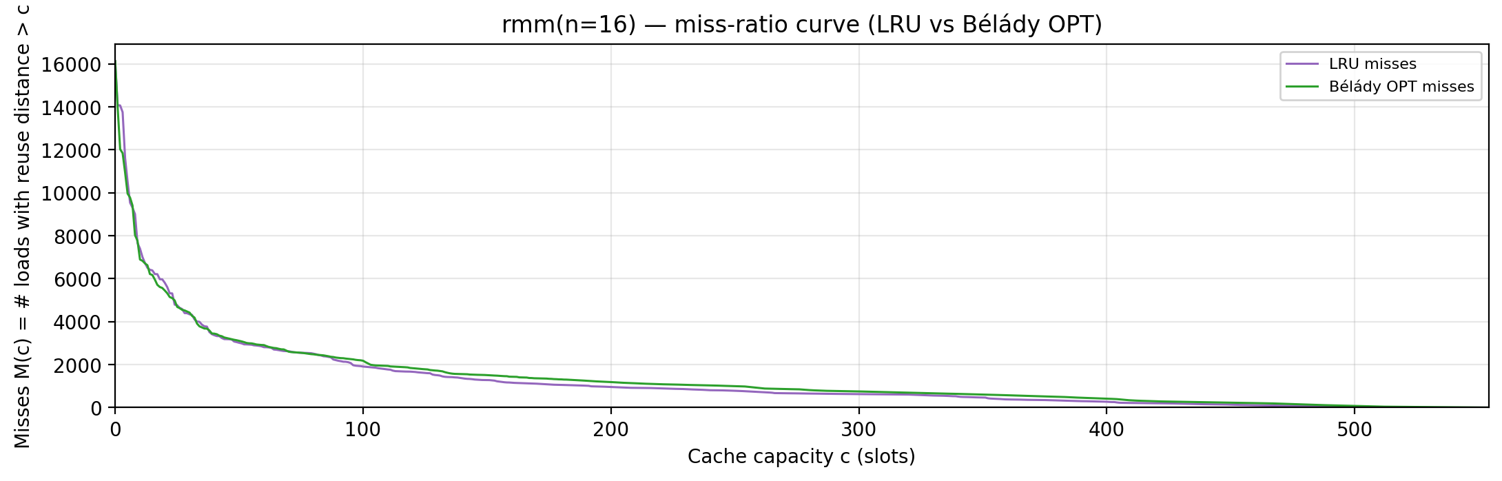
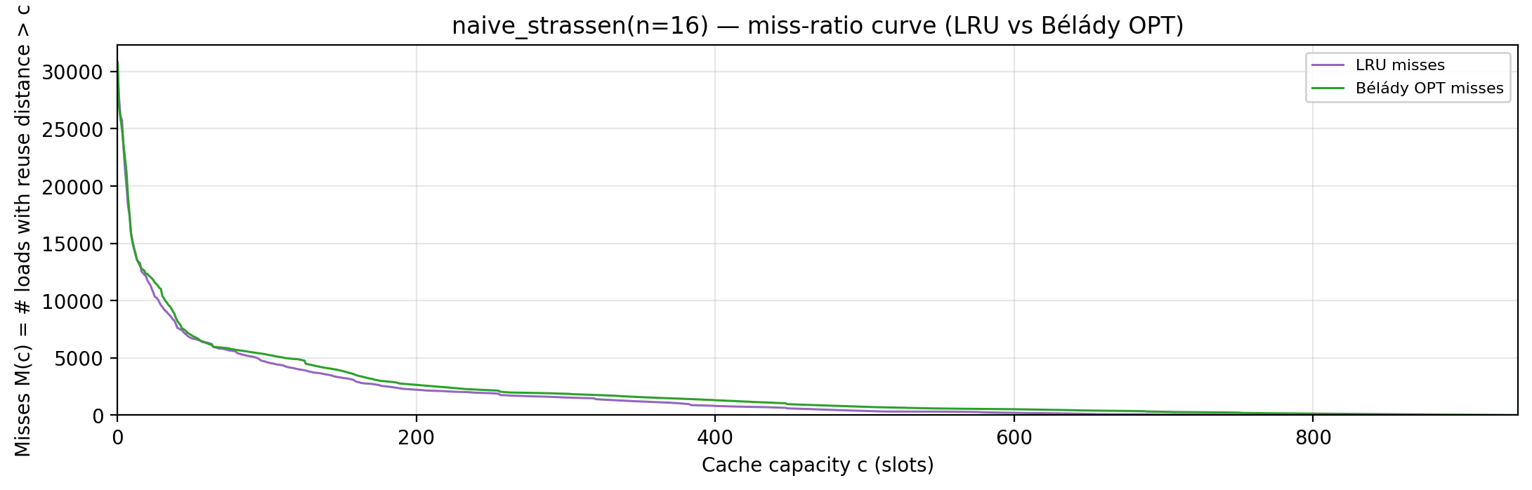
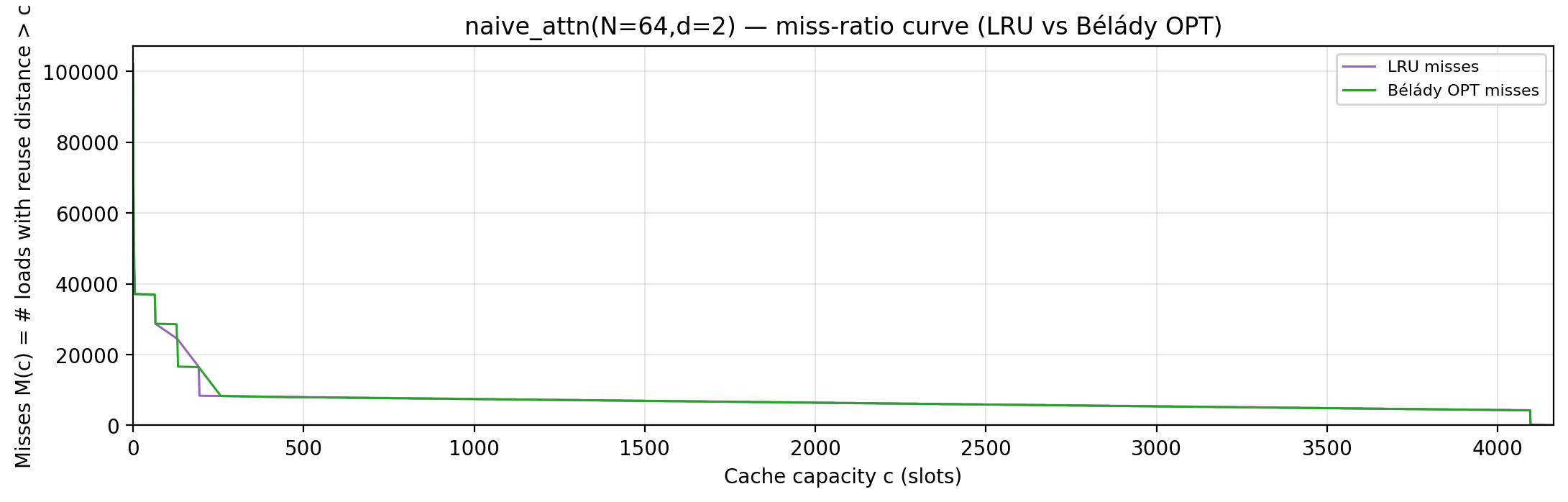
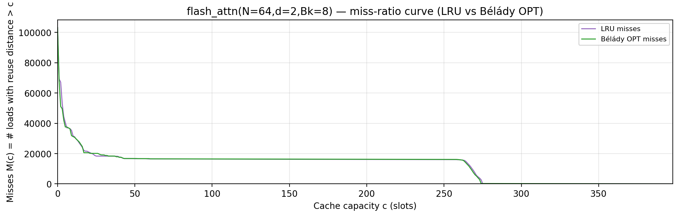
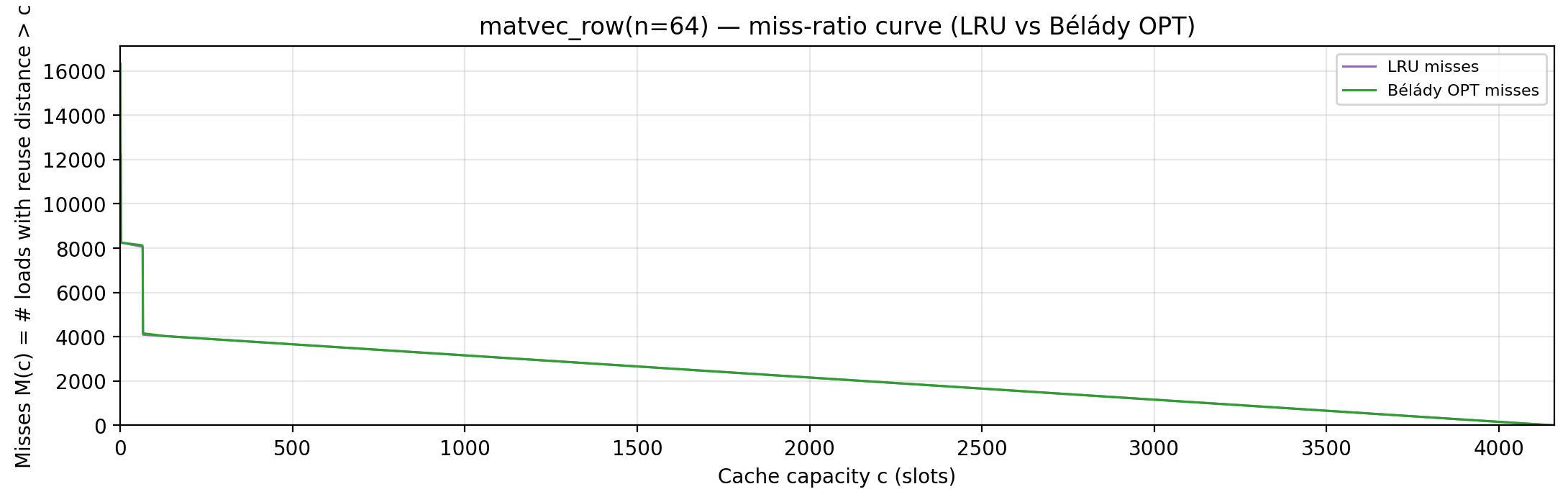
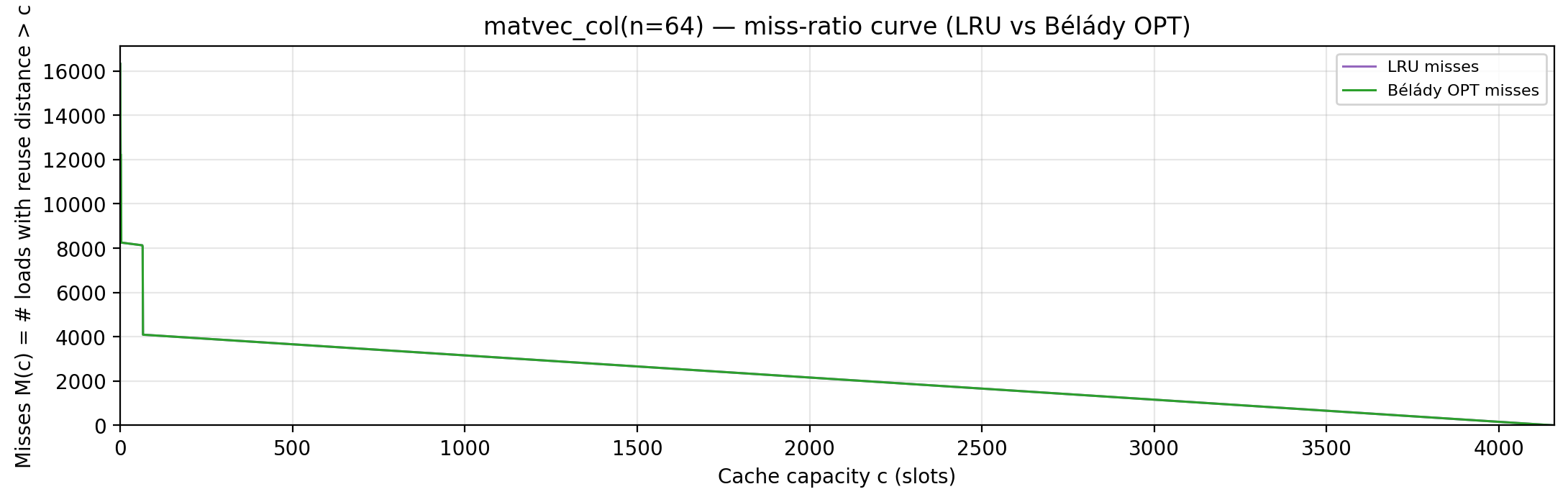
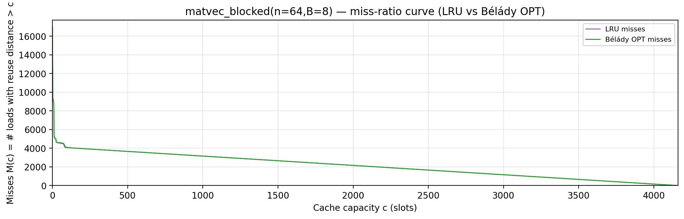
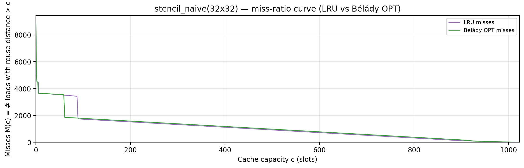
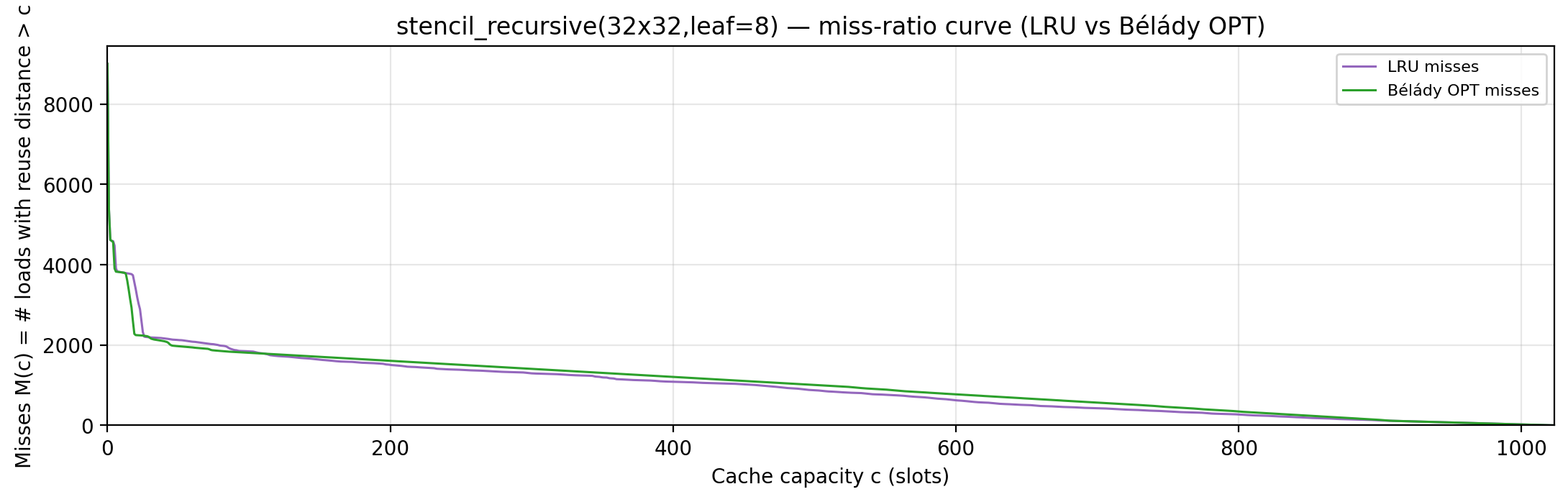
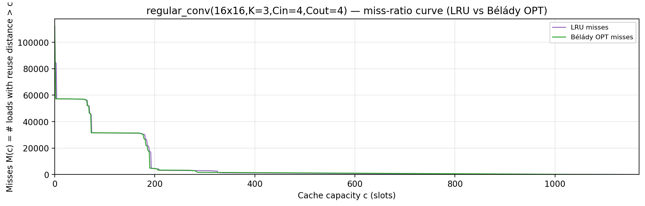
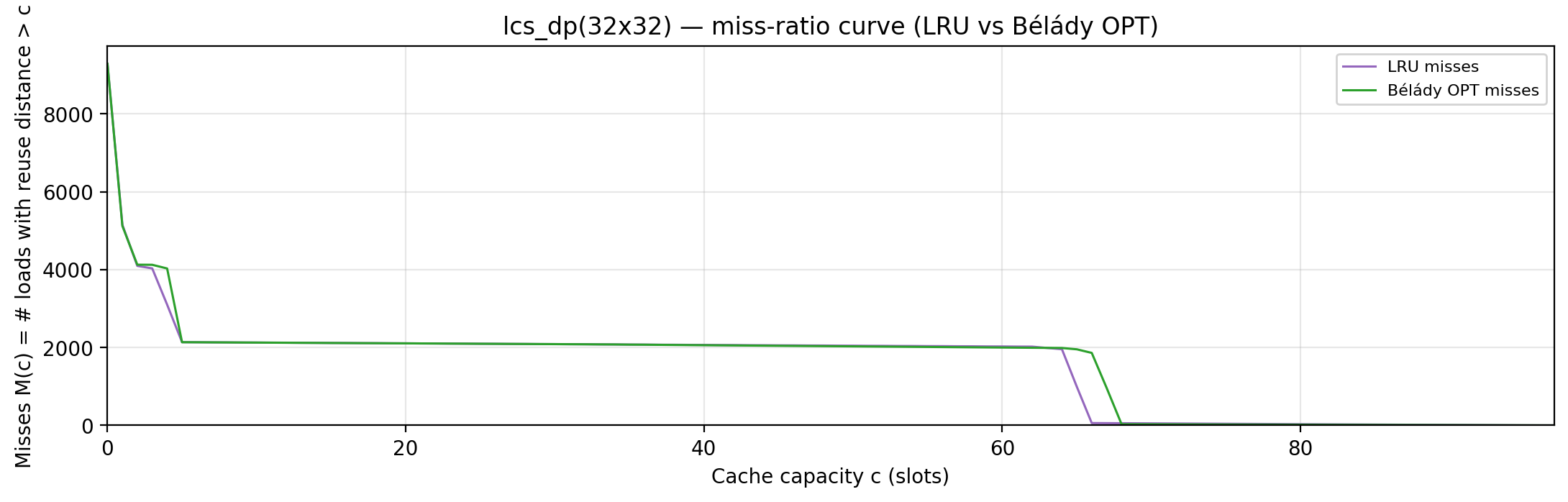
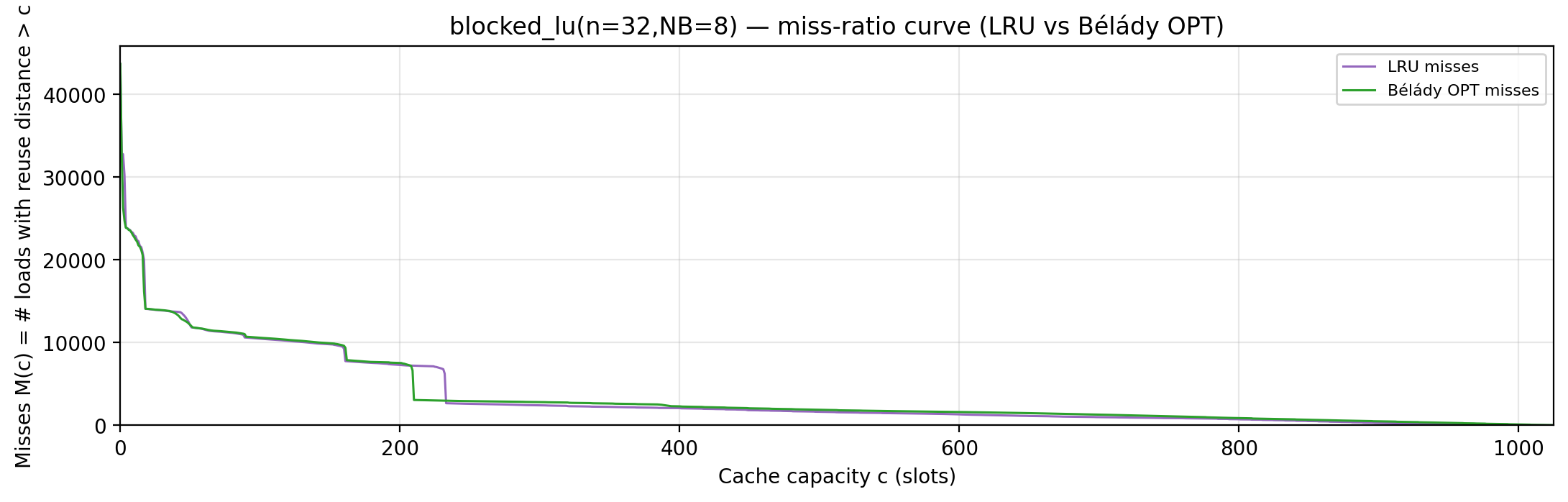
Miss-ratio curve M(c) = #loads with reuse distance > c for both LRU and OPT. The area between the curves weighted by Δ_c = ⌈√(c+1)⌉ − ⌈√c⌉ is the bytedmd_live − bytedmd_opt energy gap. |
belady-min-lower-bound.md |
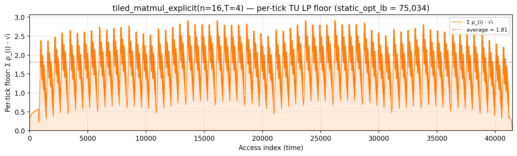
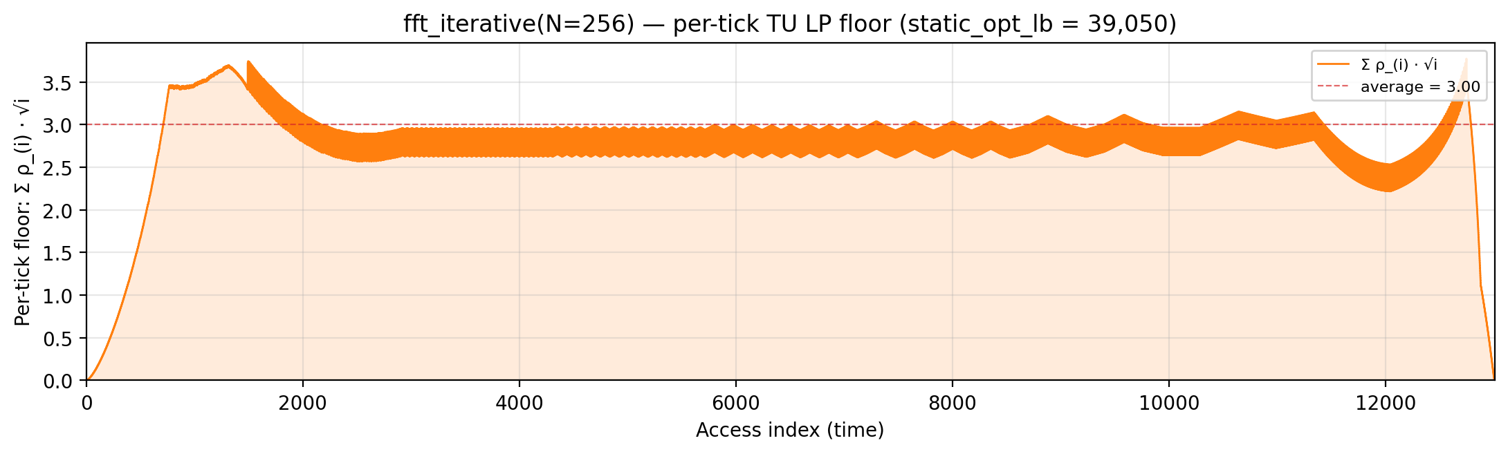
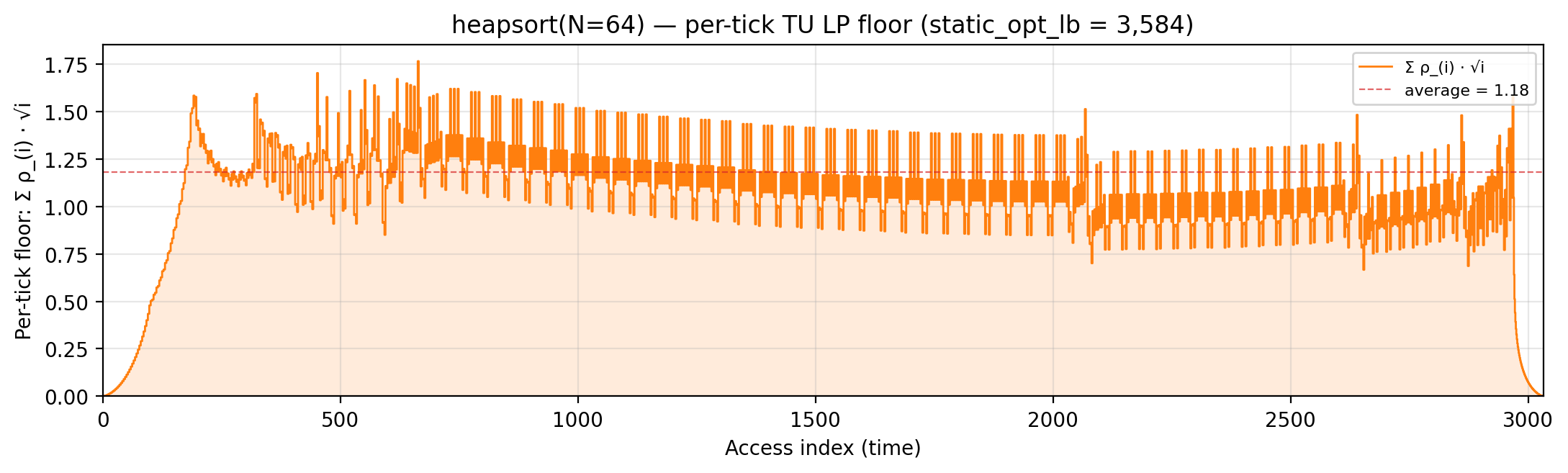
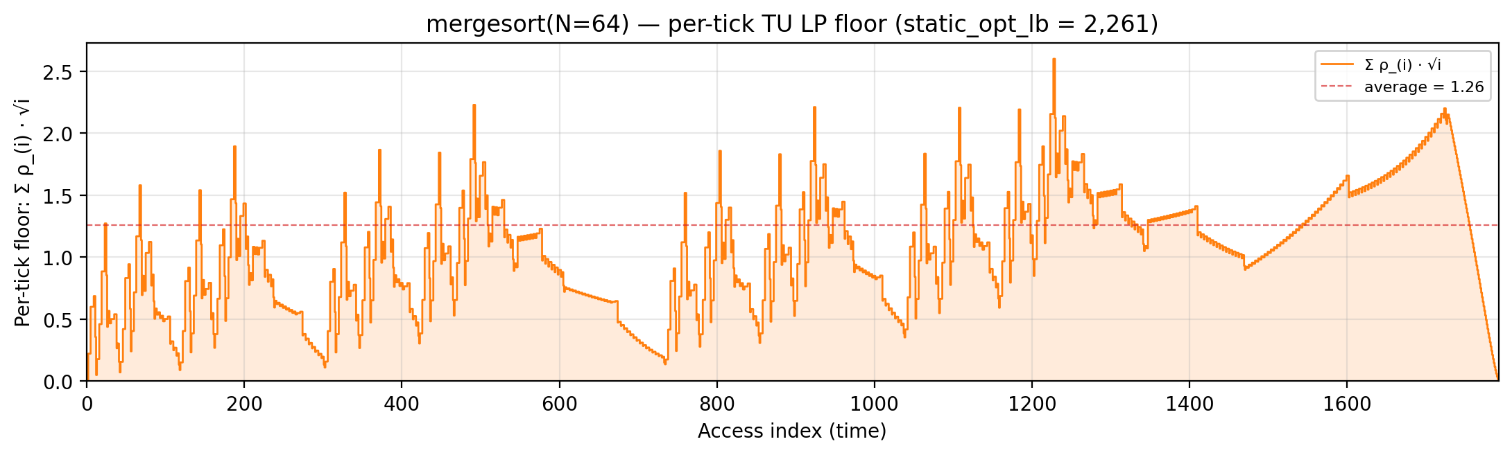
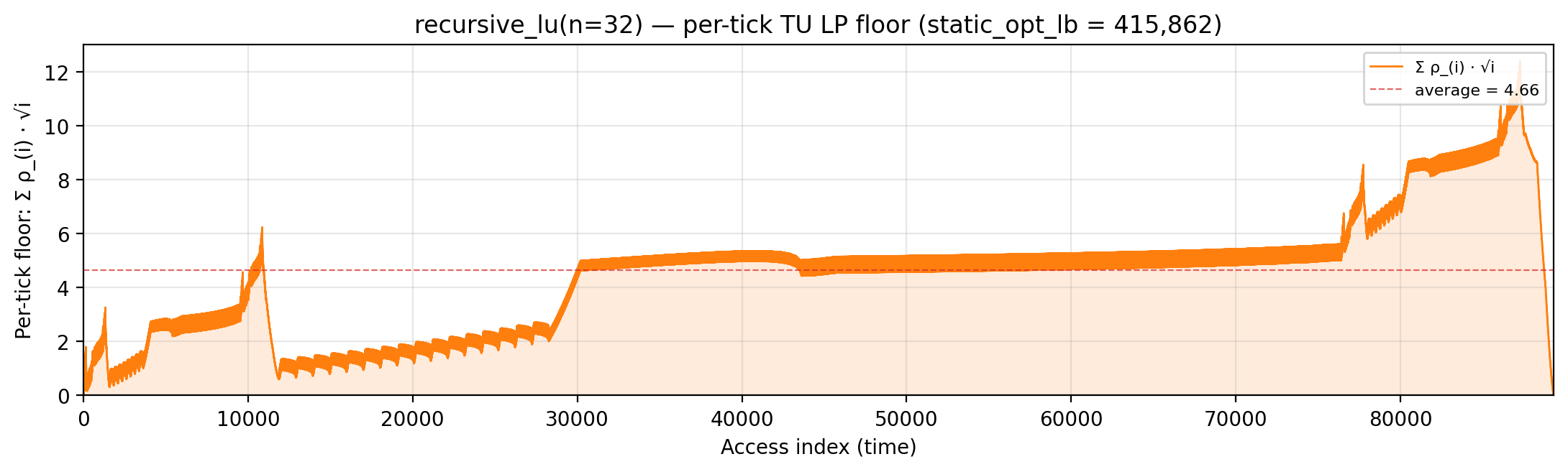
<slug>_global_density_floor.png |
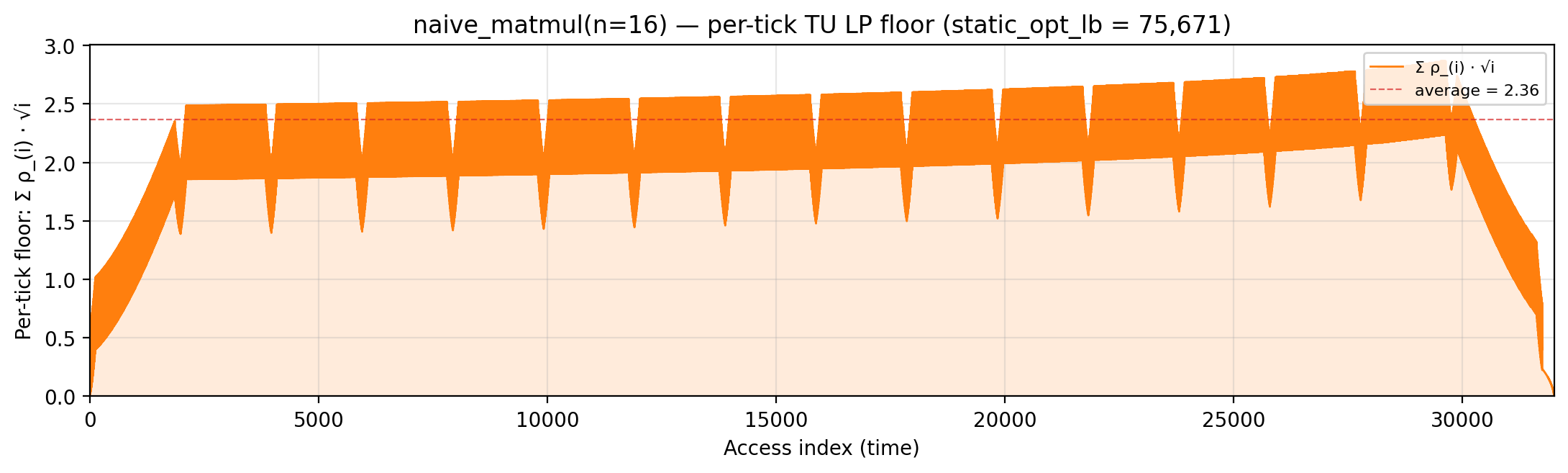
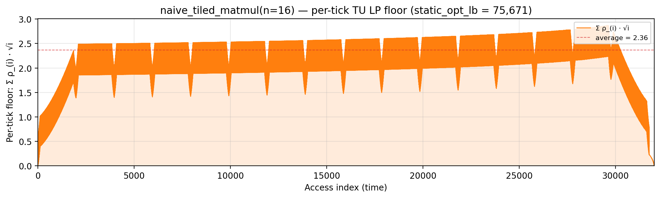
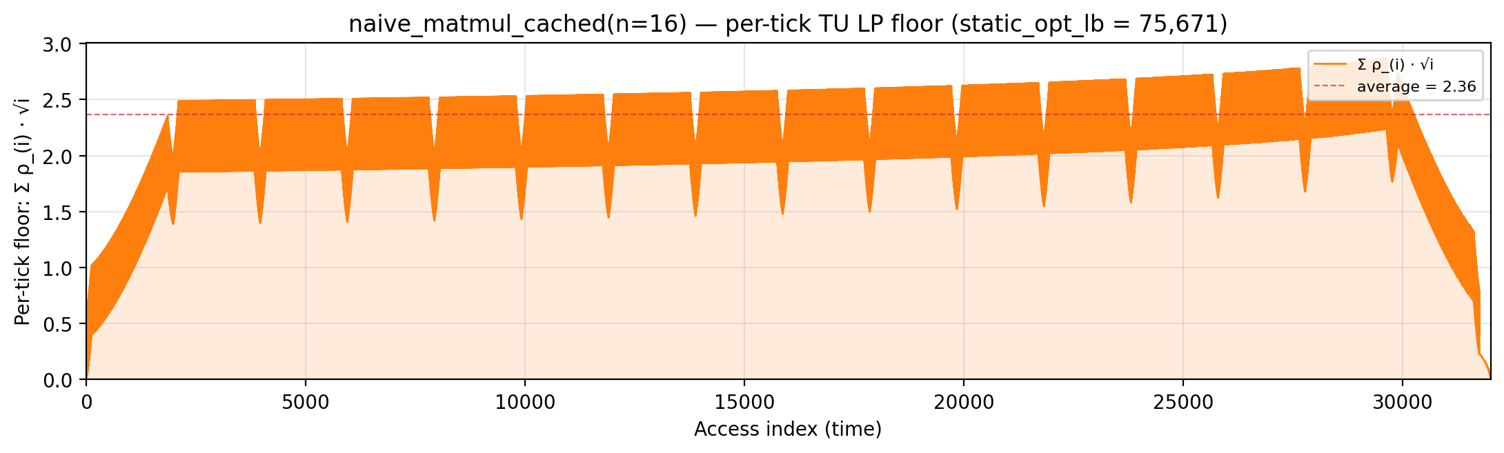
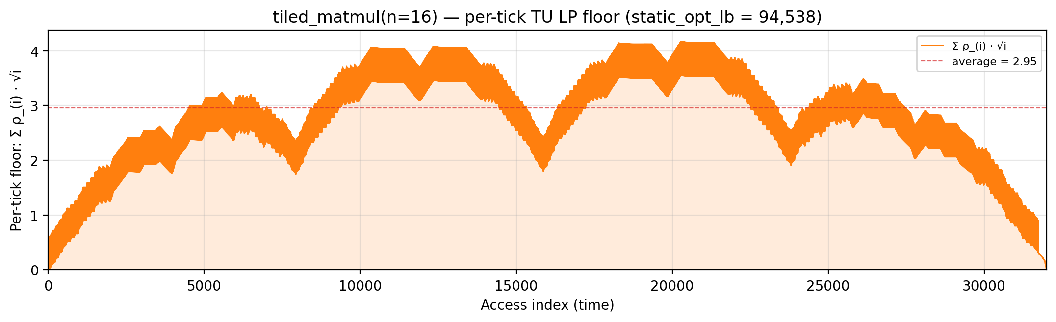
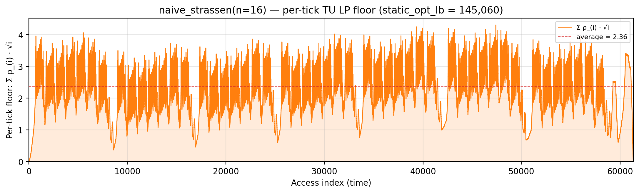
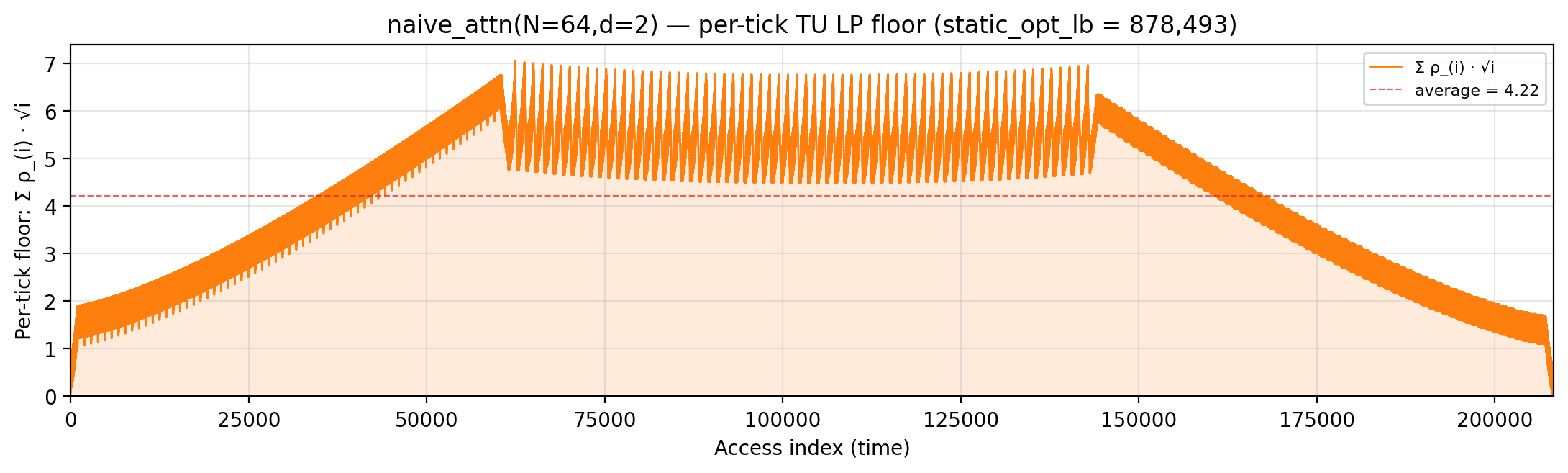
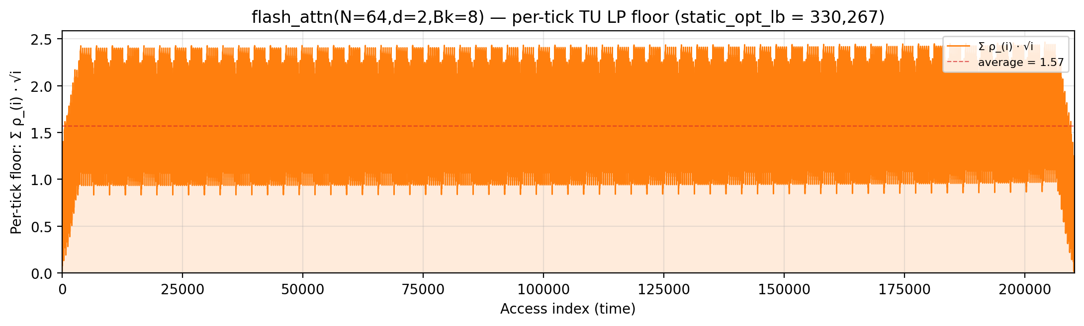
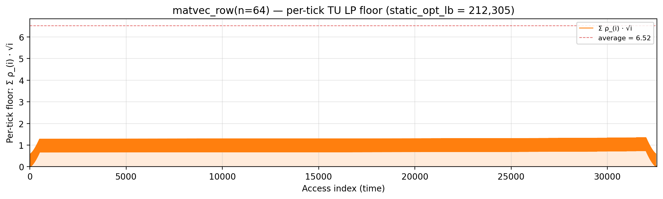
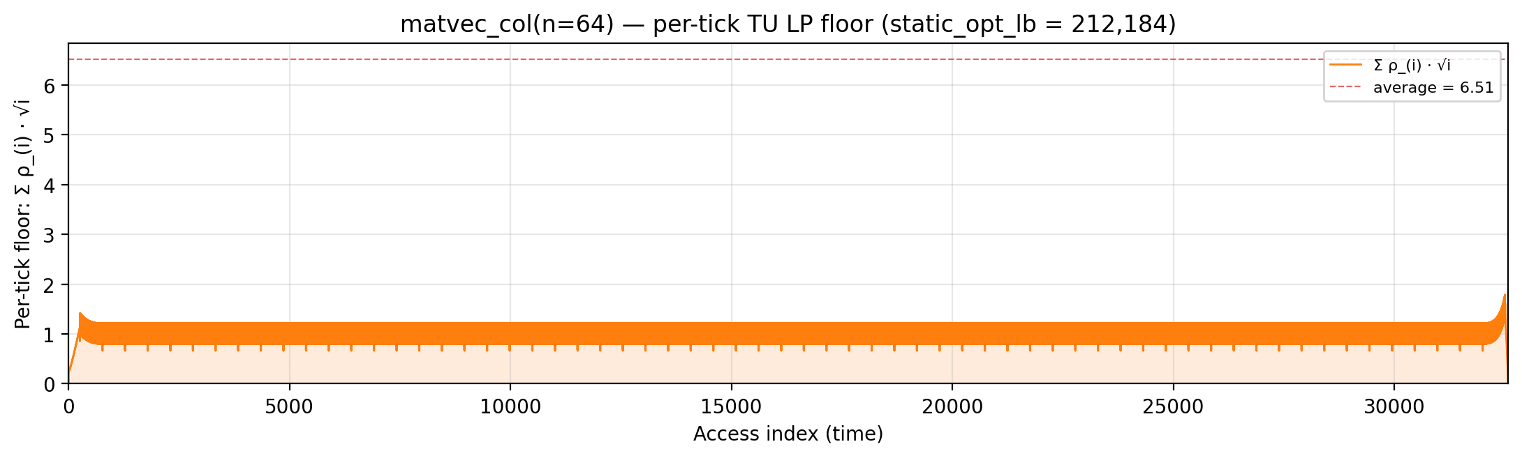
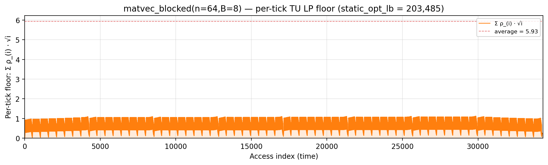
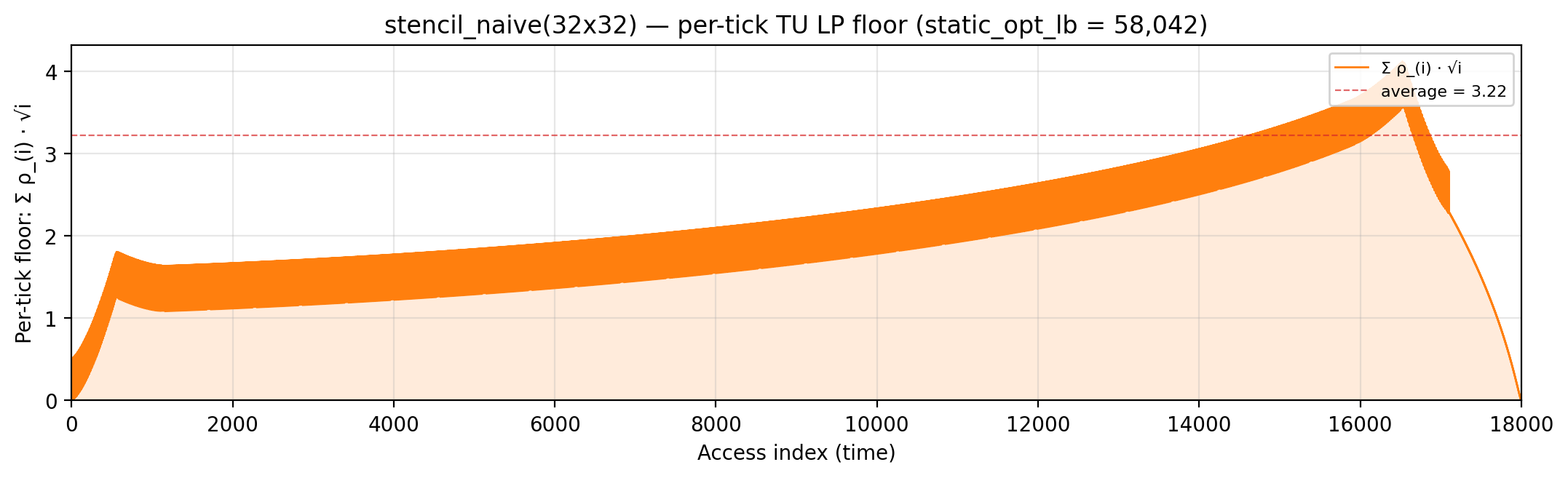
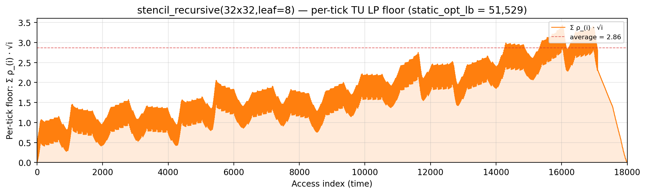
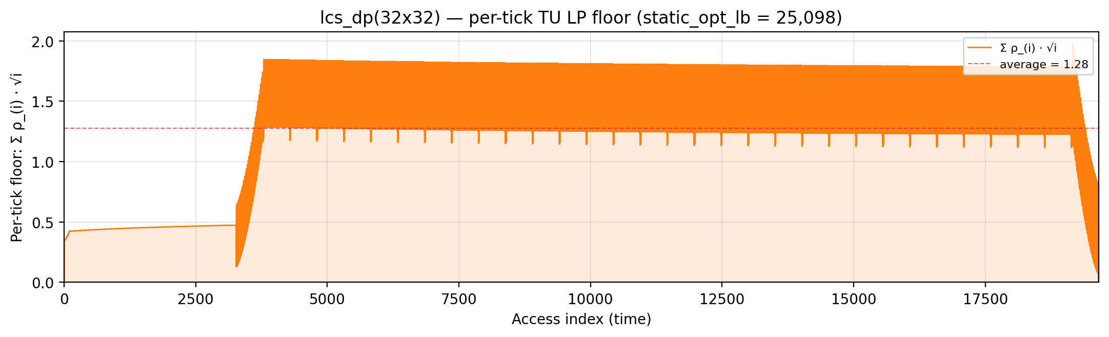
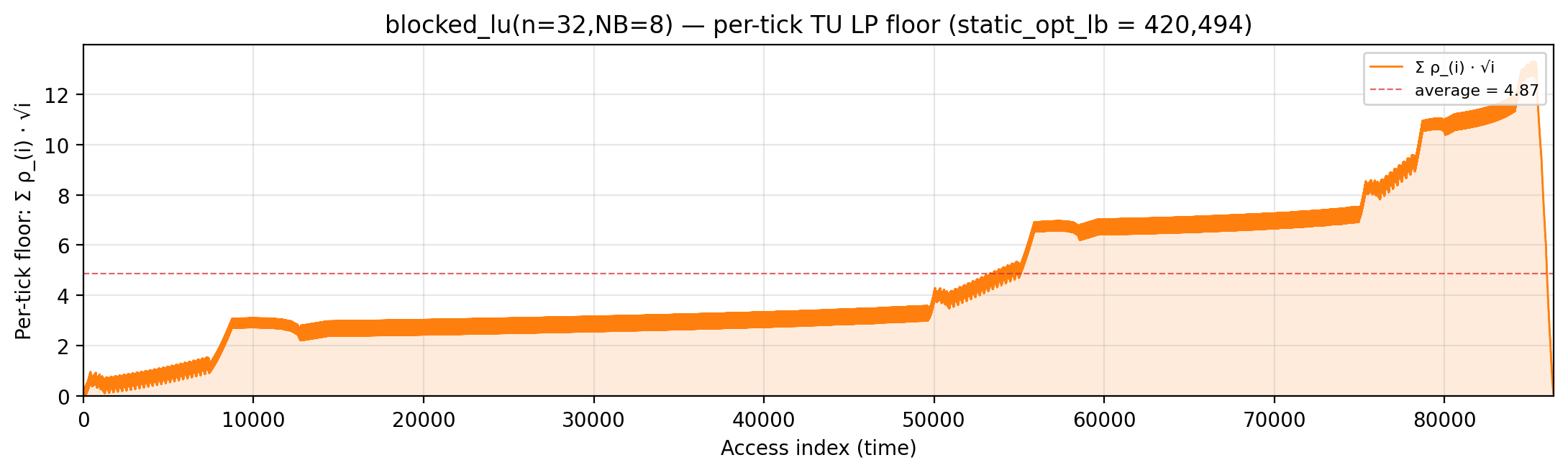
Per-tick TU LP floor Σ_i ρ_{(i)} · √i over currently-live vars (orange step curve, shaded area = global_density). Dashed red line marks the time-average. |
optimal-static-floor.md |
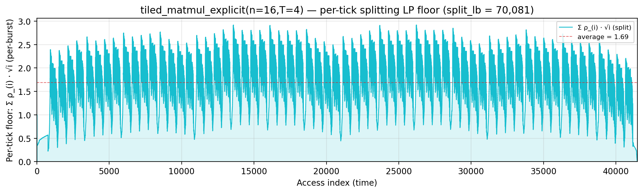
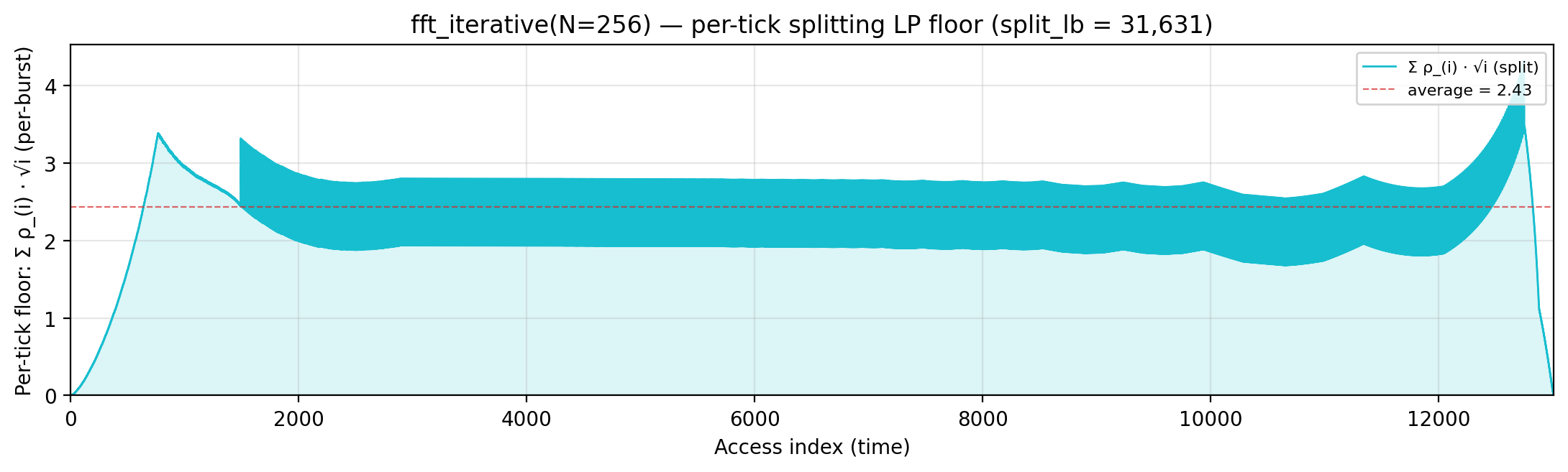
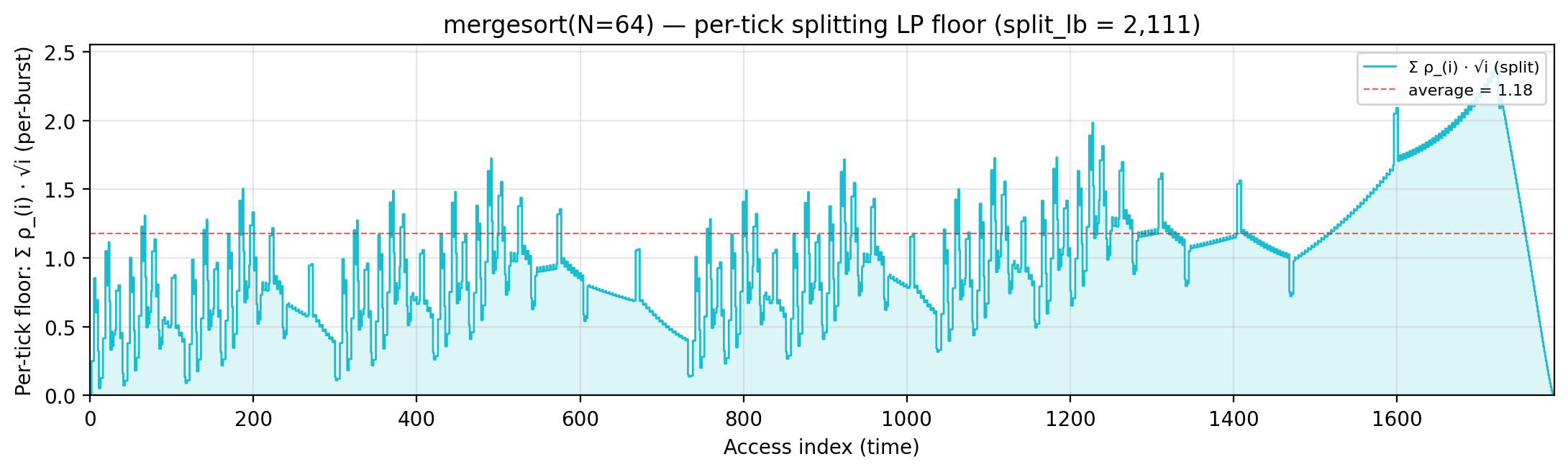
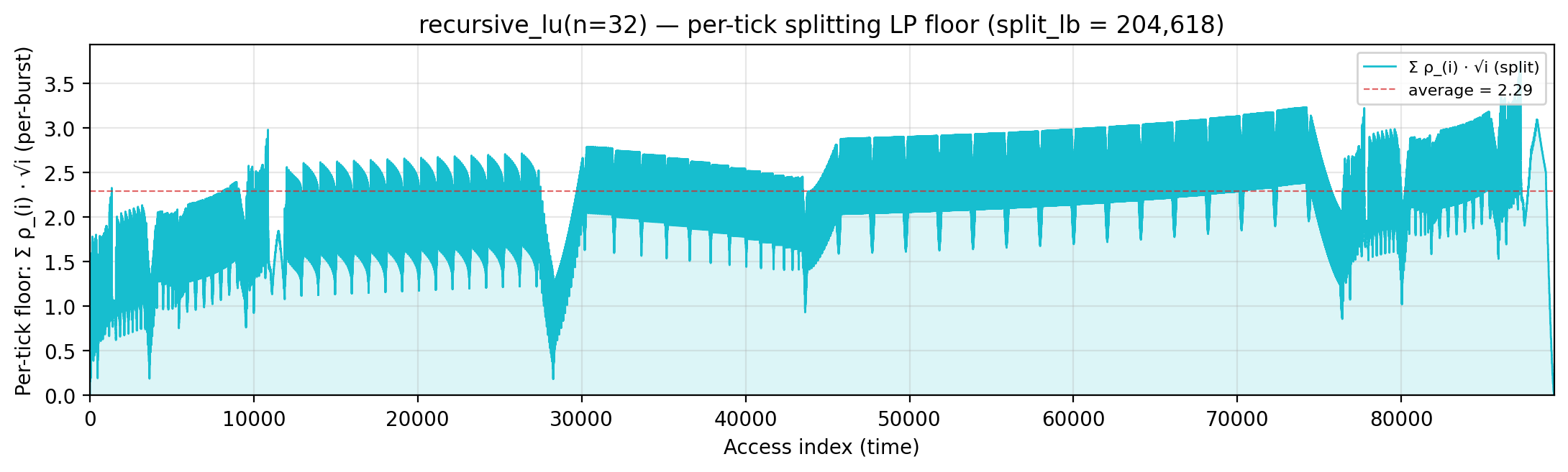
<slug>_local_density_floor.png |
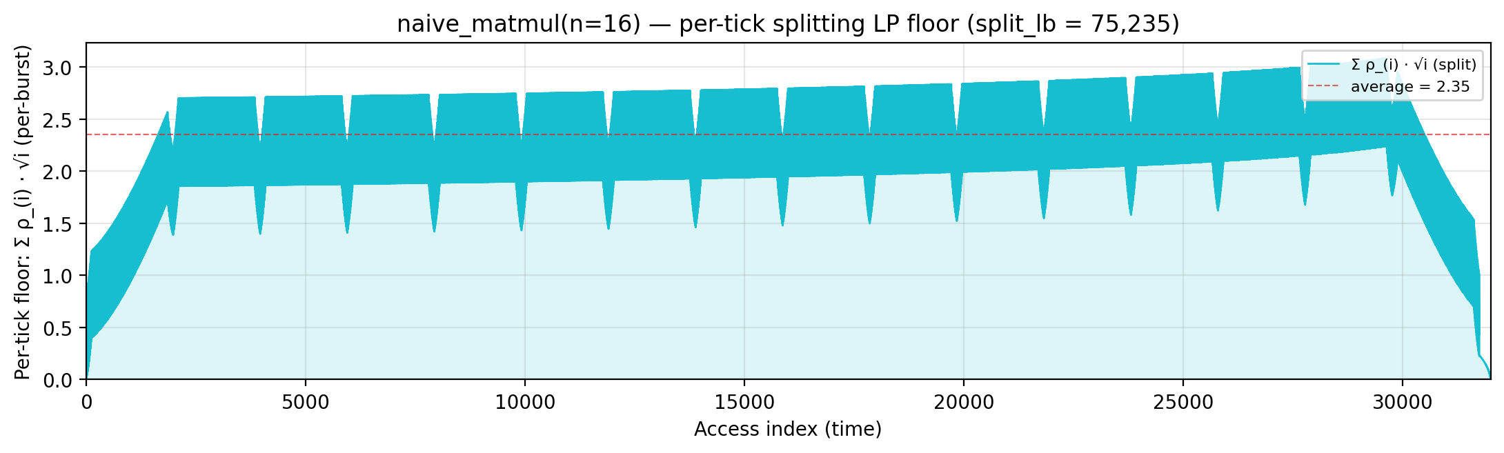
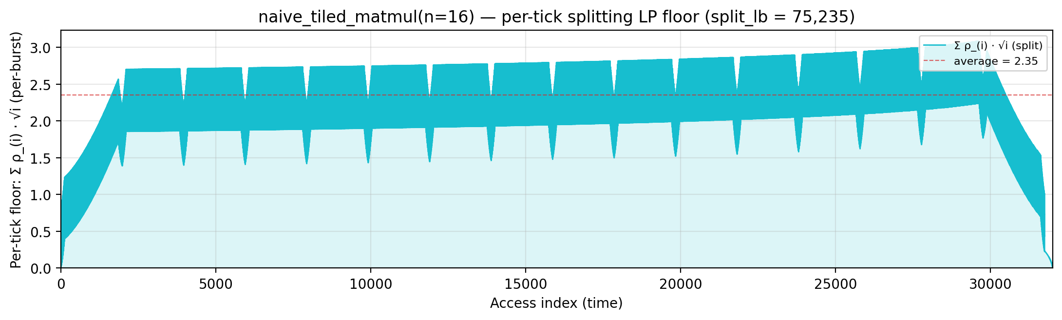
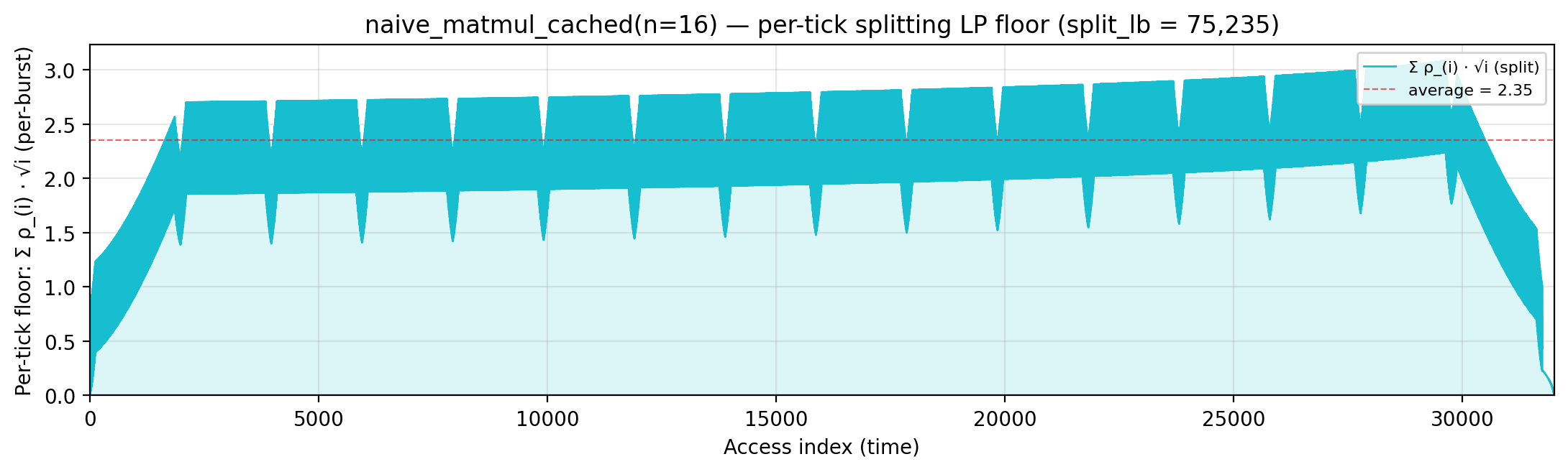
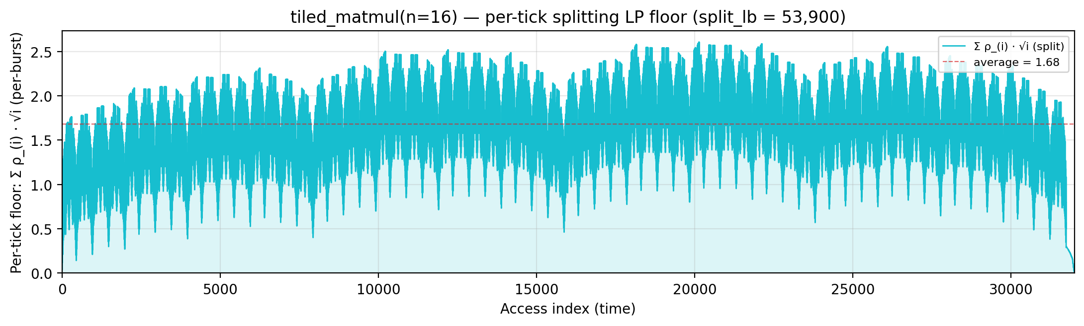
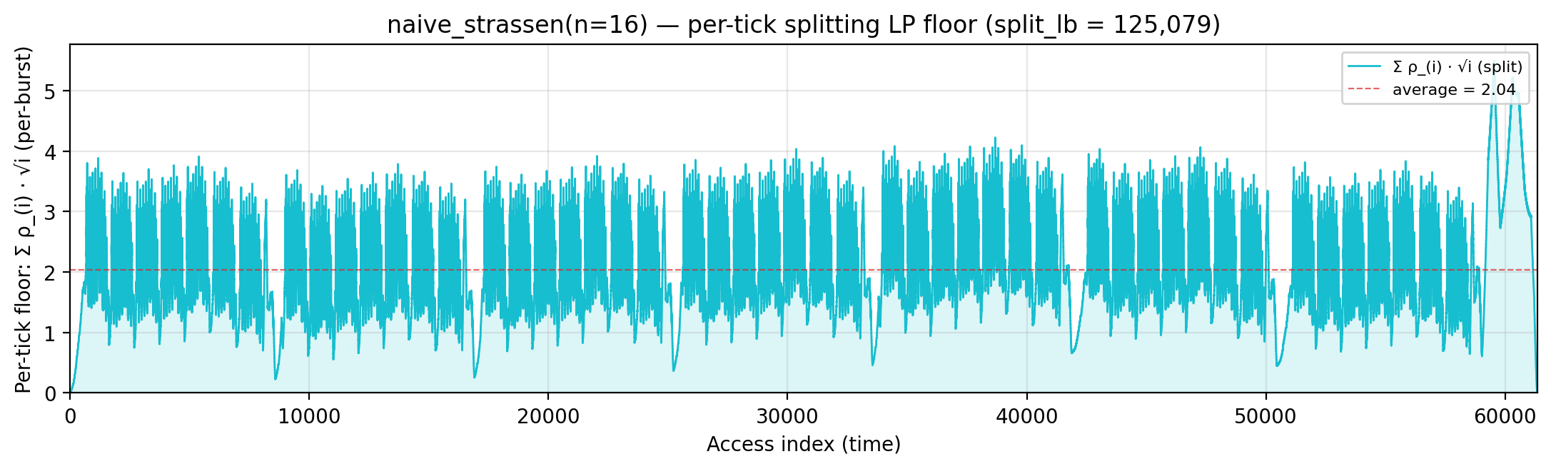
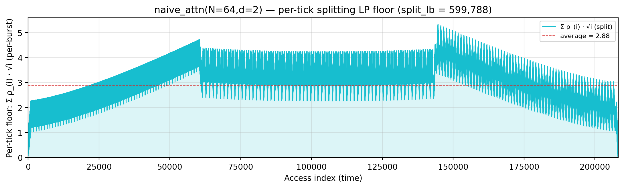
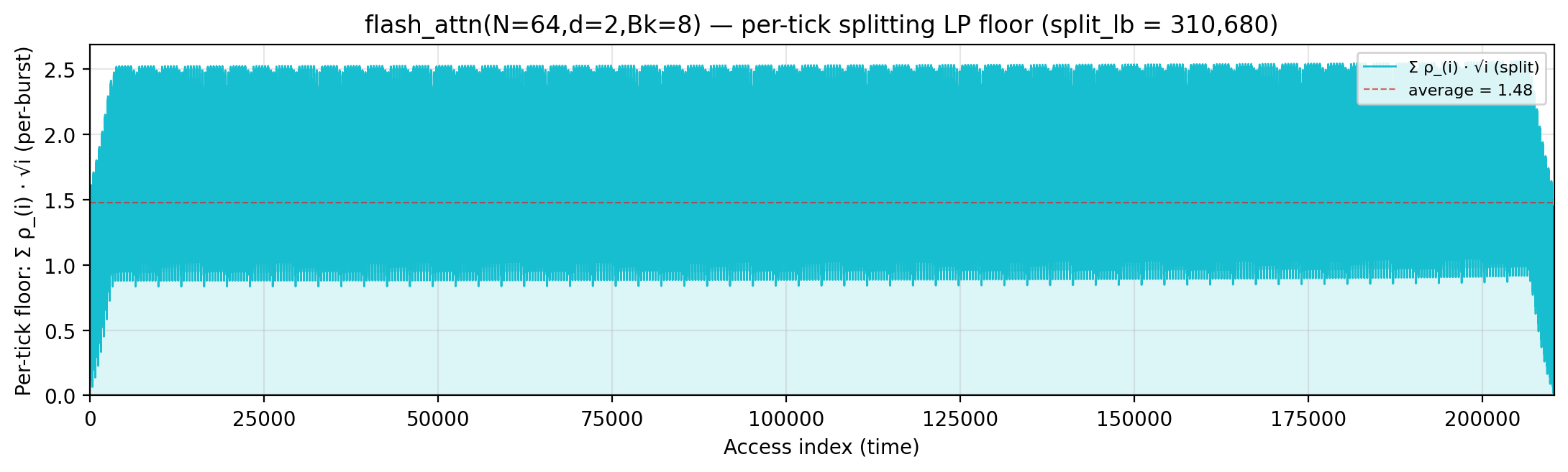
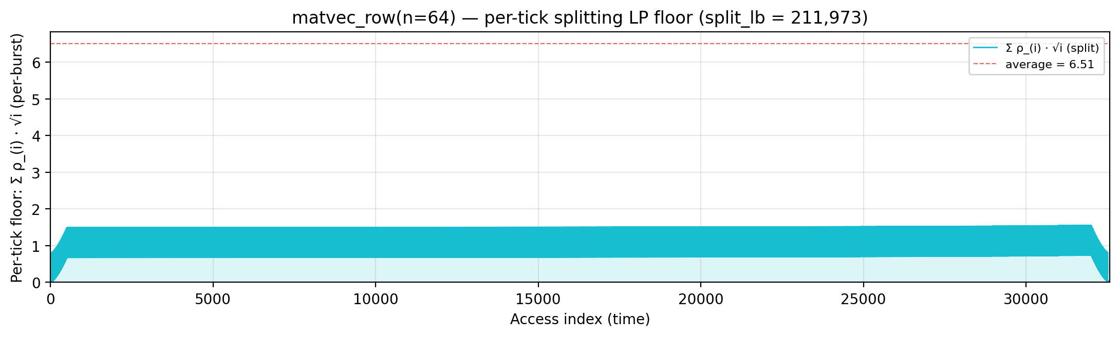
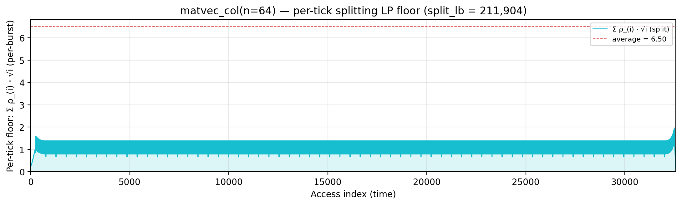
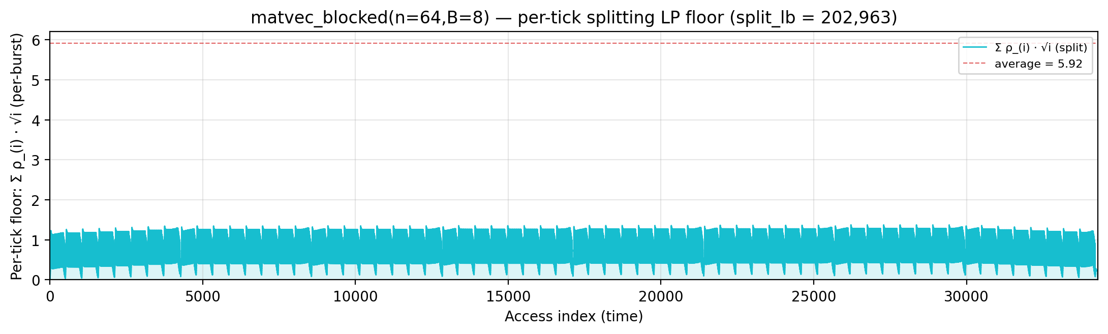
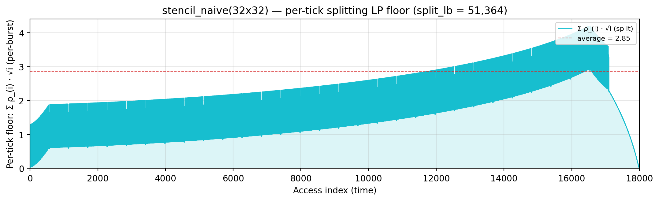
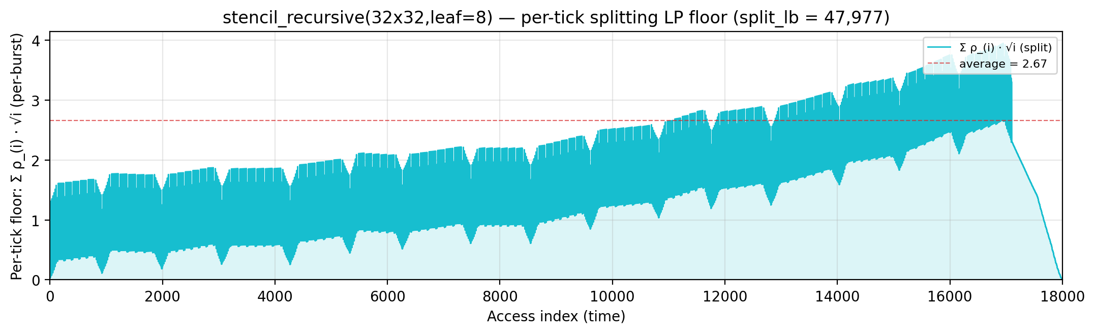
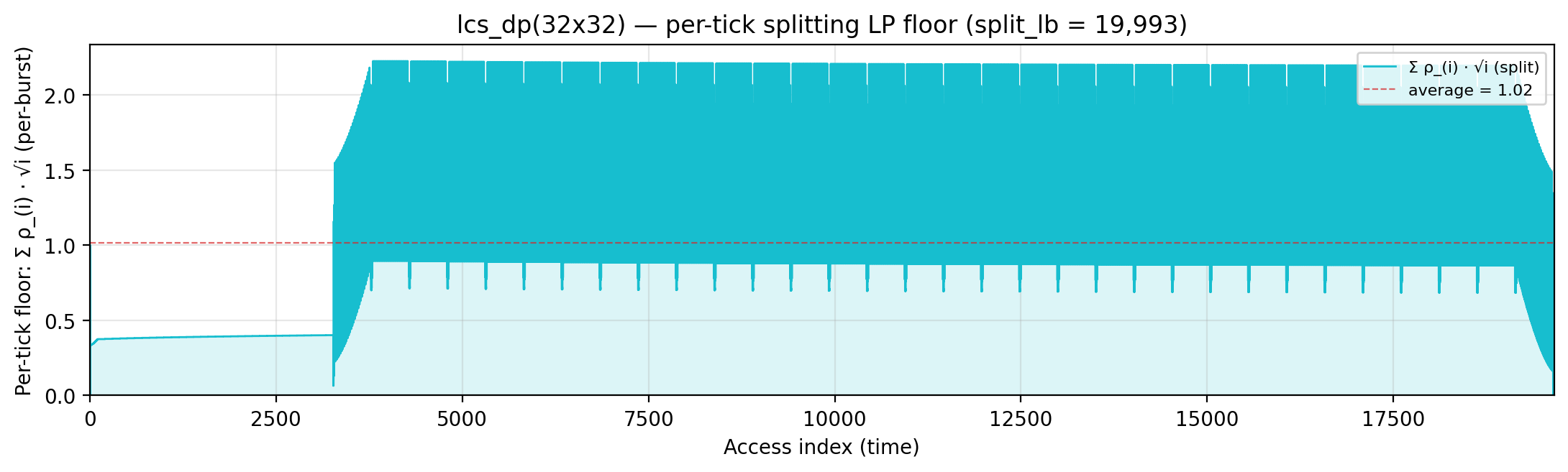
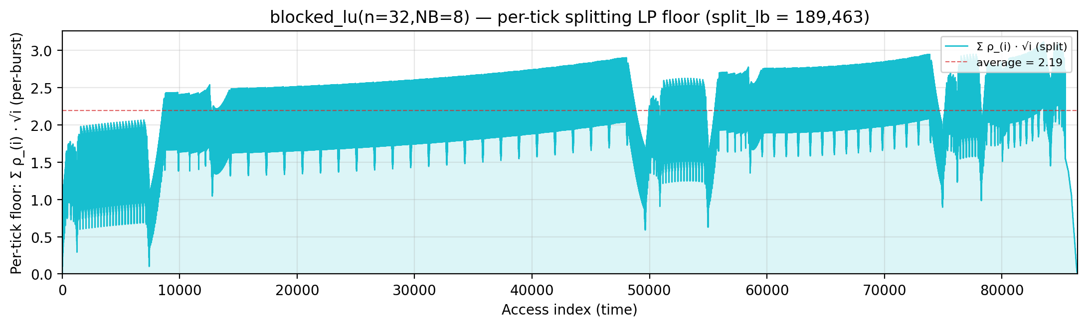
Per-tick fractional Pigeonhole floor for local_density — same Σ_i ρ_{(i)} · √i shape as _global_density_floor.png, but the entities at each tick are the per-burst virtual intervals of every variable rather than monolithic per-variable lifespans (cyan step curve, shaded area = the geometric portion of local_density). On phase-structured traces a long dormant burst gets a low ρ → high rank → small per-tick contribution, so this curve sits below _global_density_floor.png. |
fractional-lp-splitting.md |
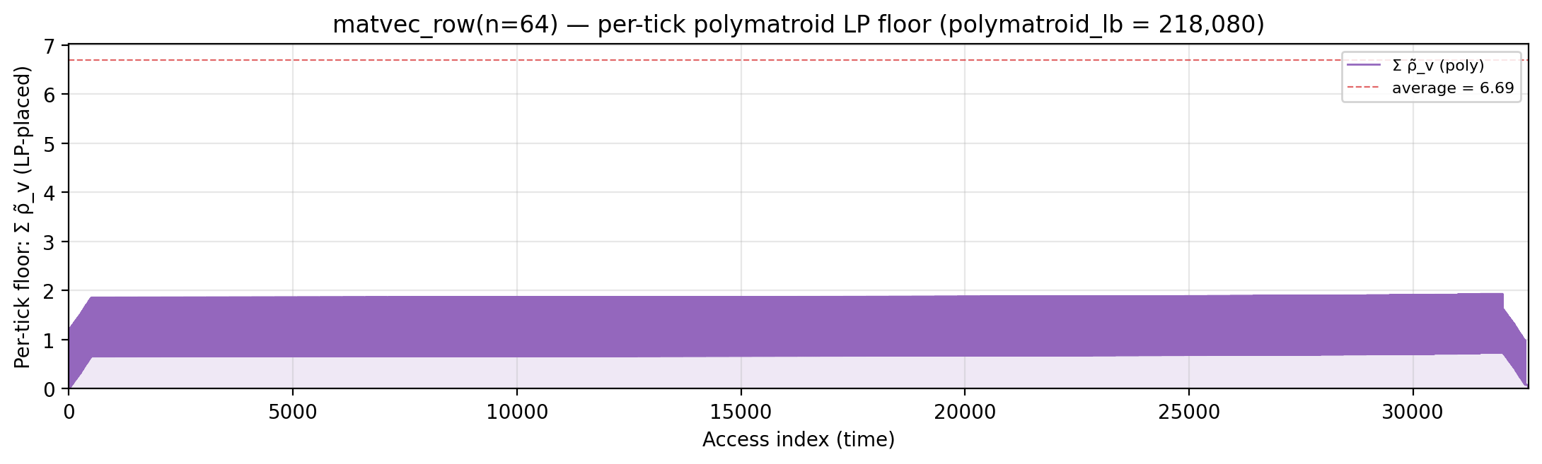
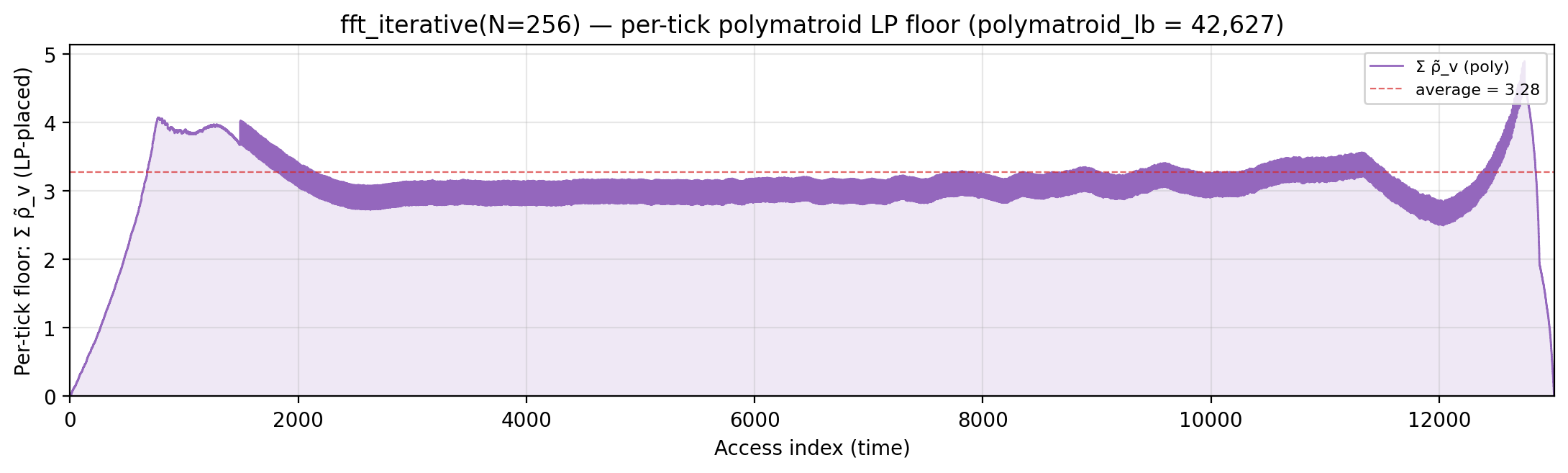
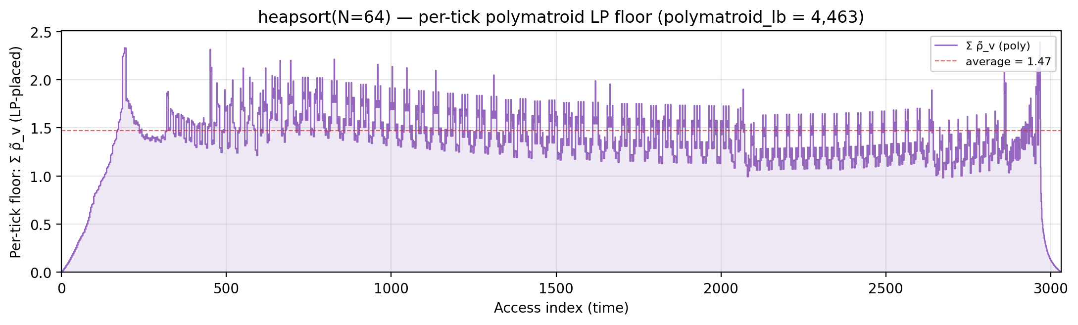
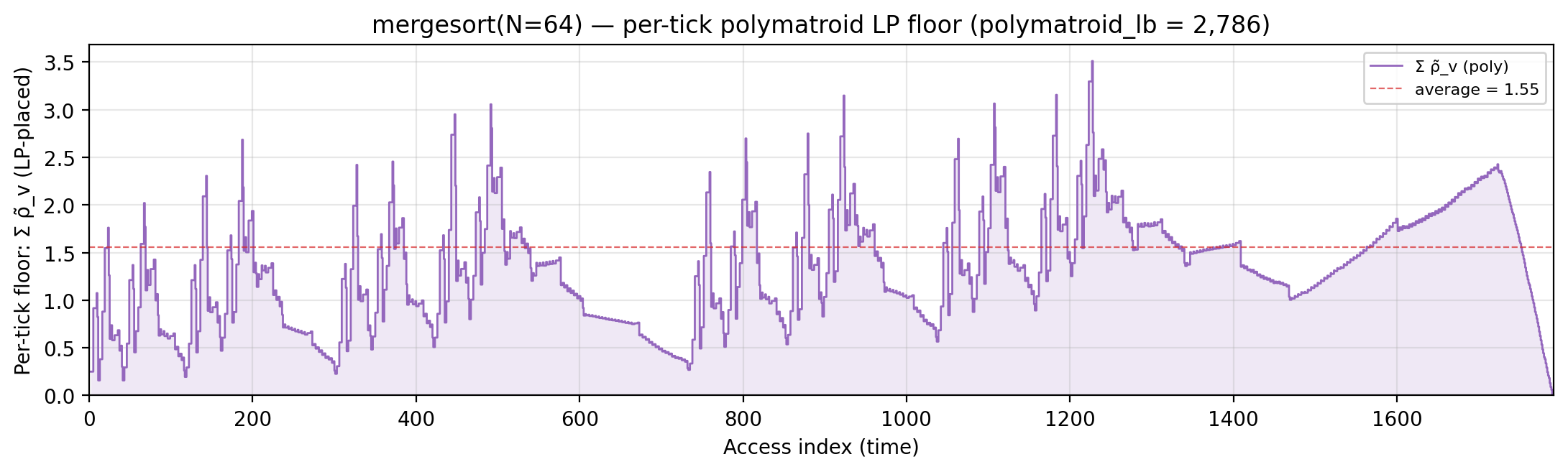
<slug>_polymatroid_floor.png |
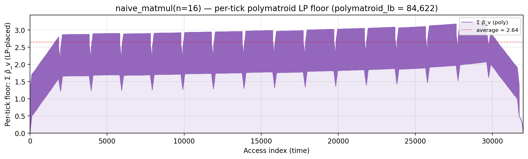
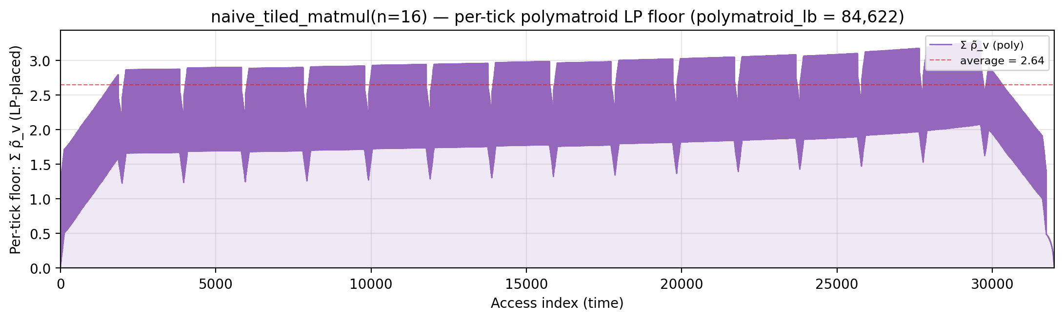
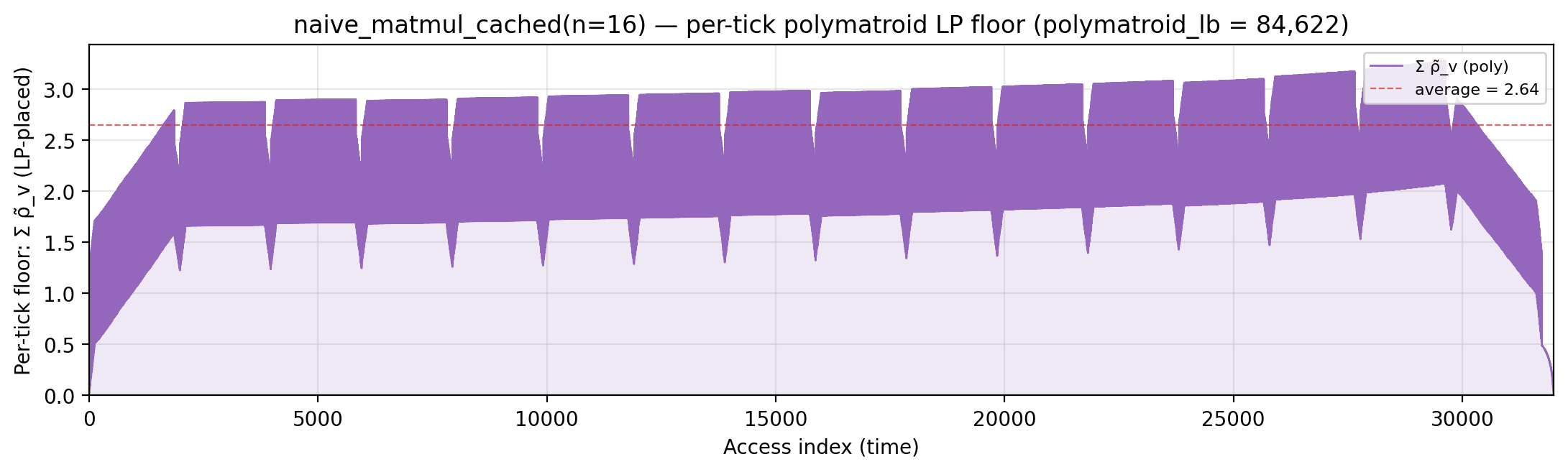
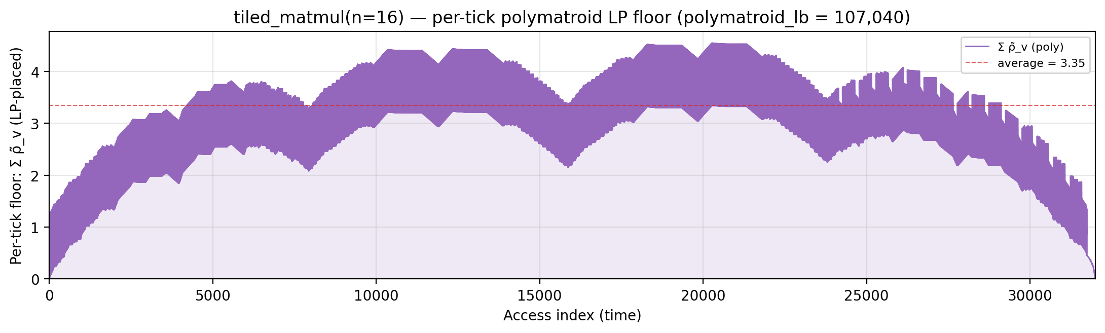
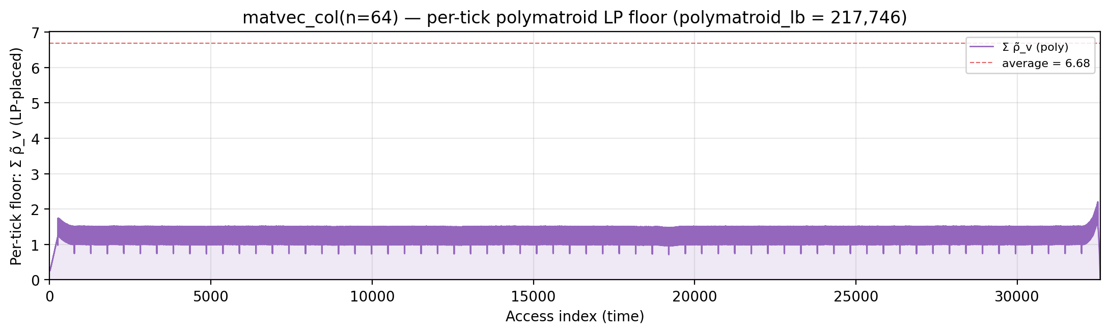
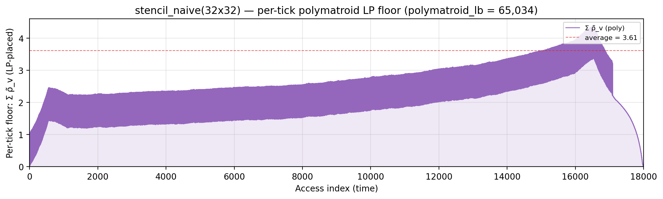
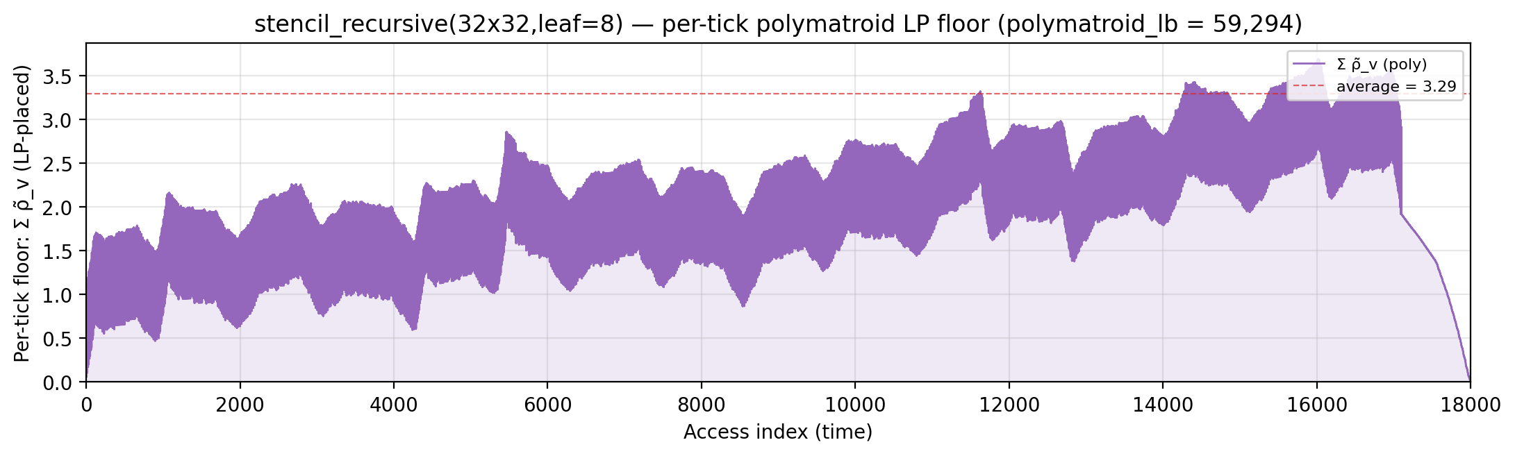
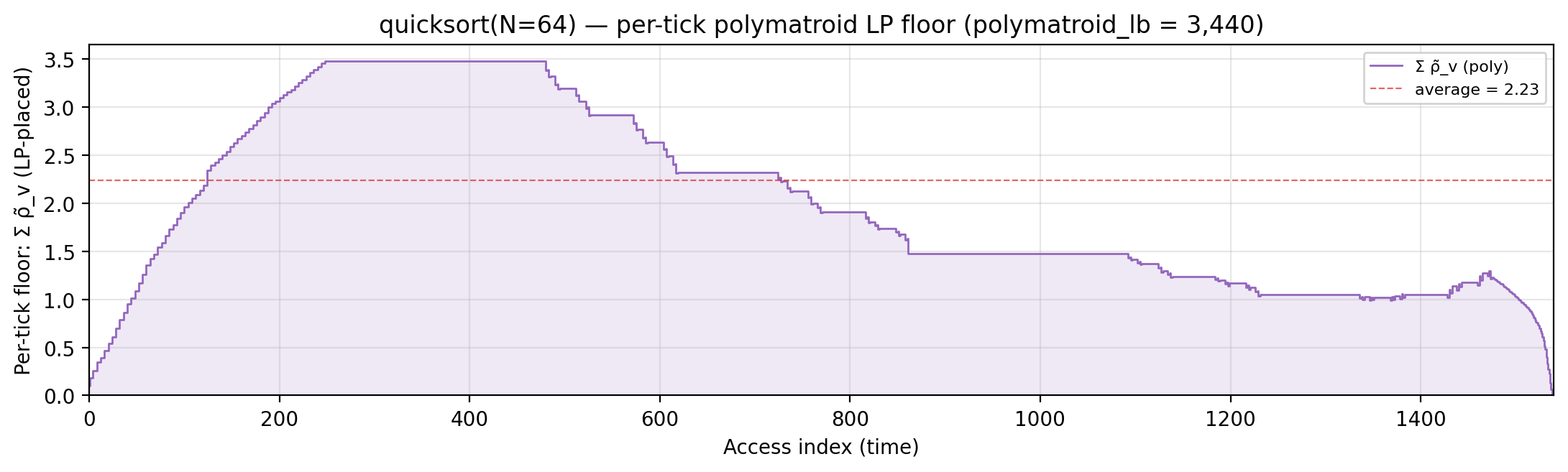
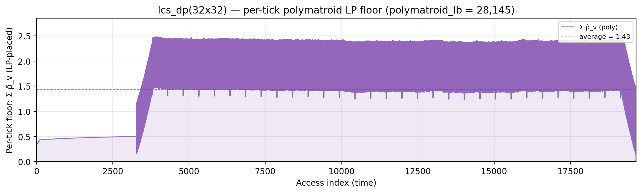
Per-tick polymatroid LP floor Σ_v ρ̃_v over live vars, where each variable’s LP-implied depth d_v = min{c² : v ∈ S_{c²}} from the discrete polymatroid LP gives ρ̃_v = reads(v) · ⌈√d_v⌉ / lifespan(v) (purple step curve, shaded area = the geometric portion of polymatroid_lb). Models the rigid-spatial-lock-in regime, so this curve sits above _global_density_floor.png whenever both render. Skipped when the LP exceeds the 30 s wall-time budget or the row hits the events ≤ 100k AND peak_live ≤ 1000 pre-screen — that excludes LU/QR/Cholesky/Strassen/attention/transpose/spatial+regular conv. |
polymatroid-relaxation.md |
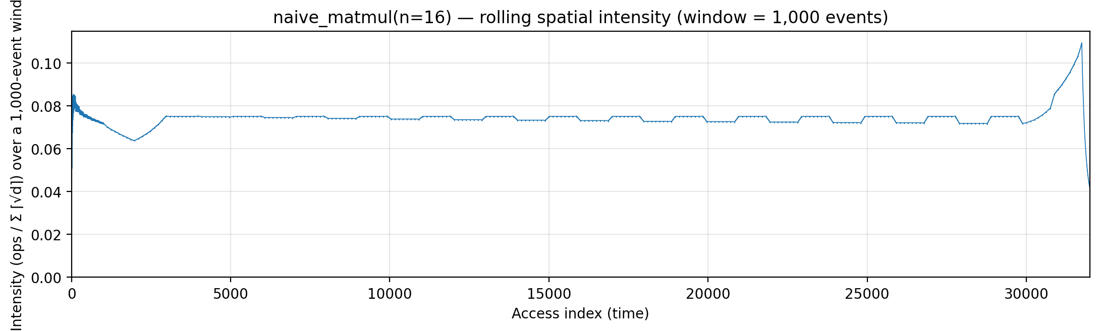
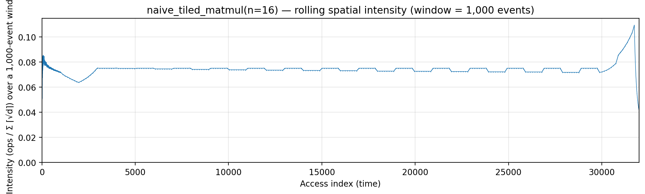
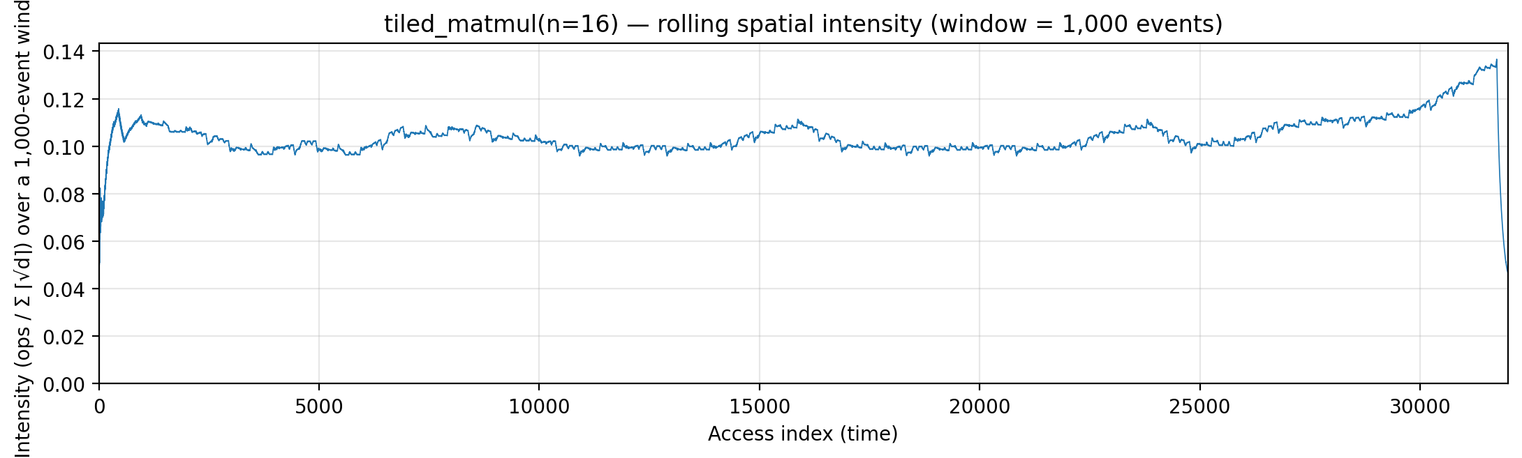
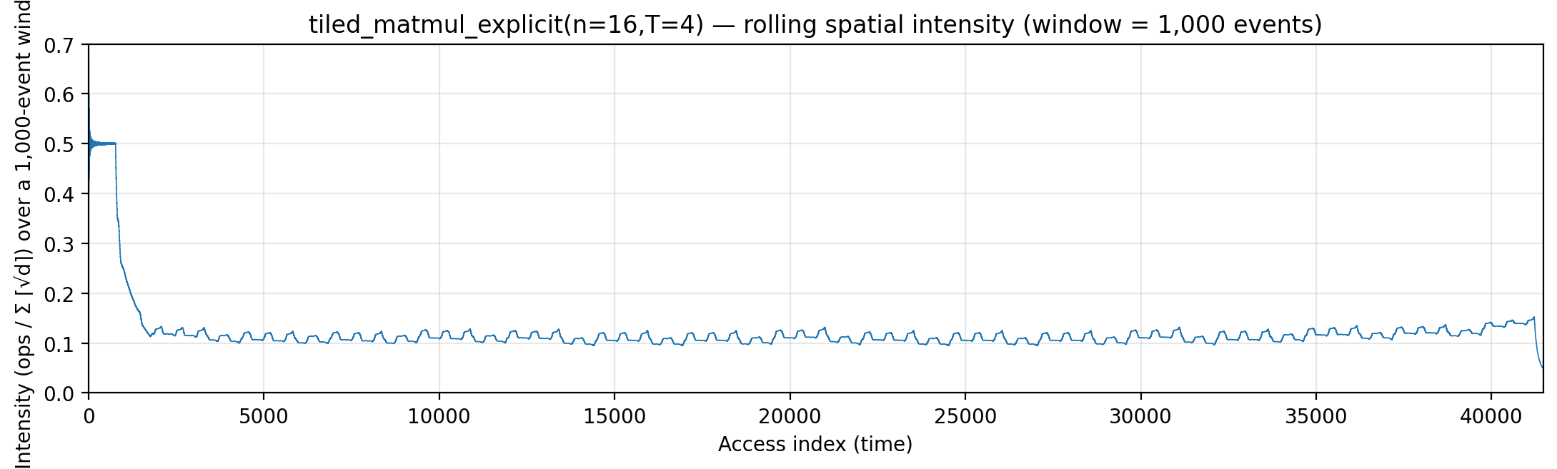
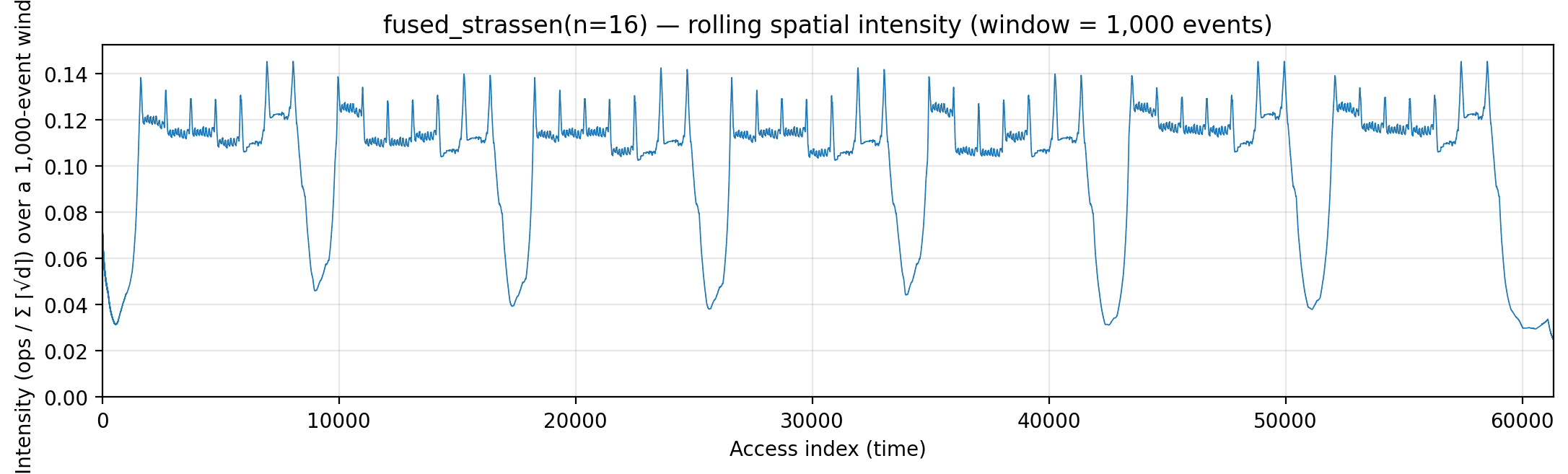
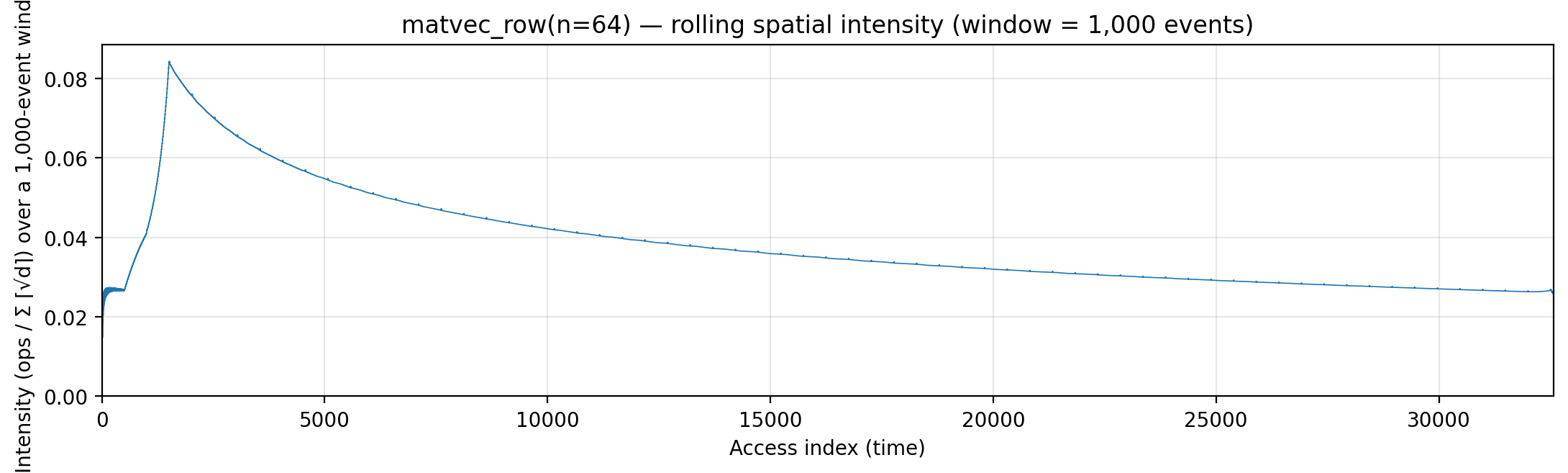
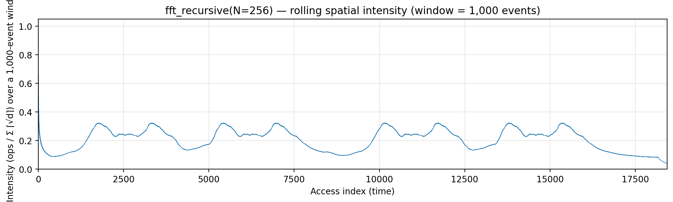
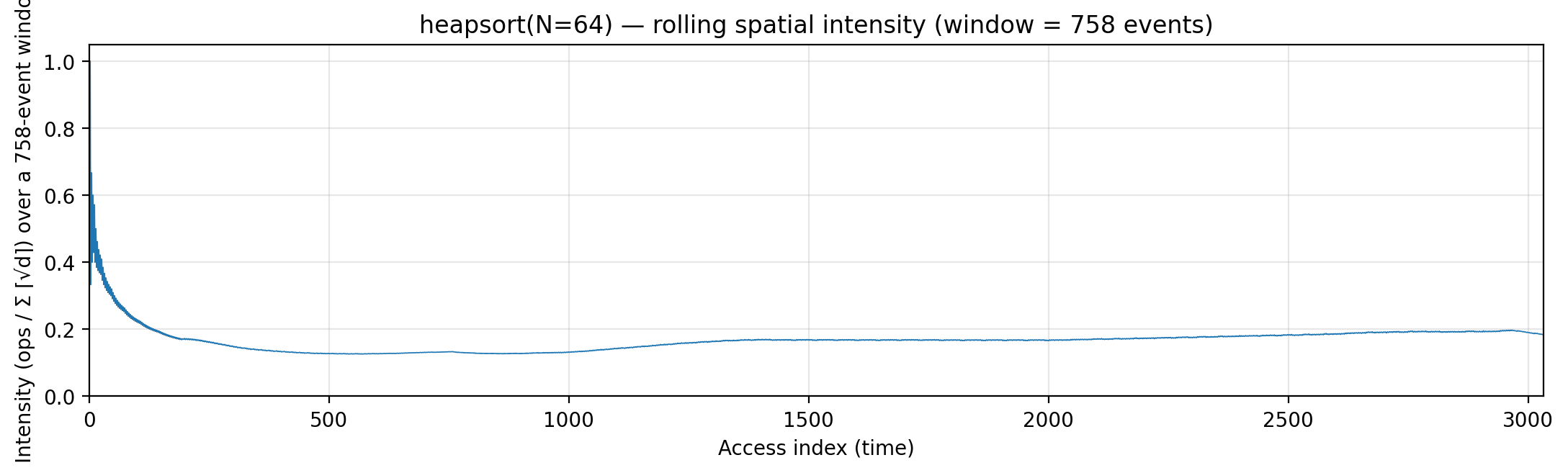
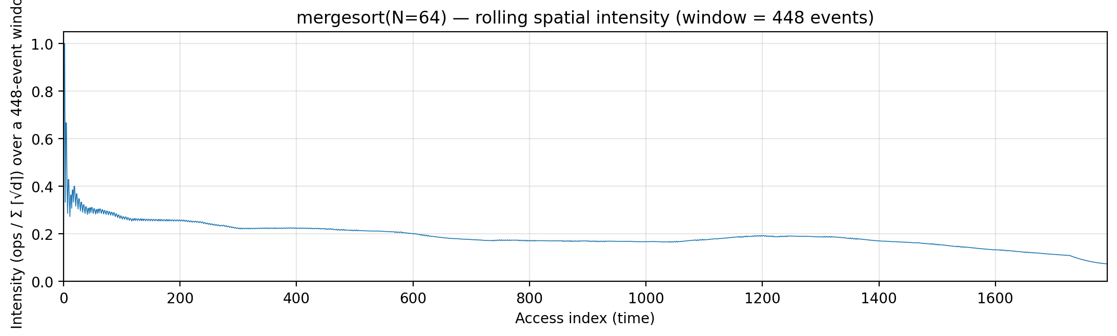
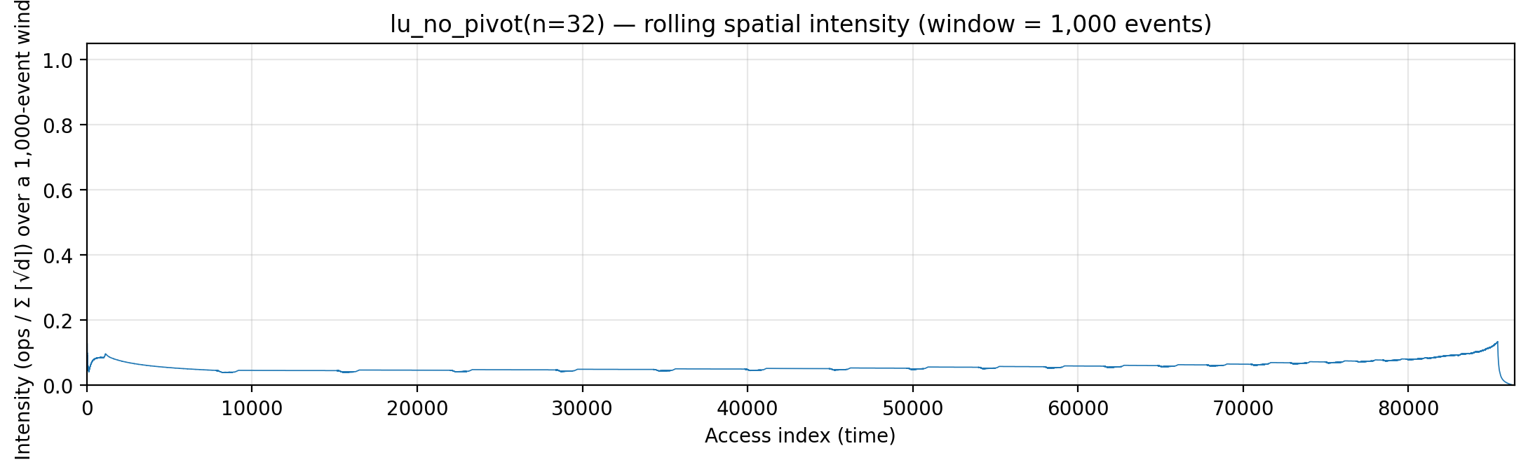
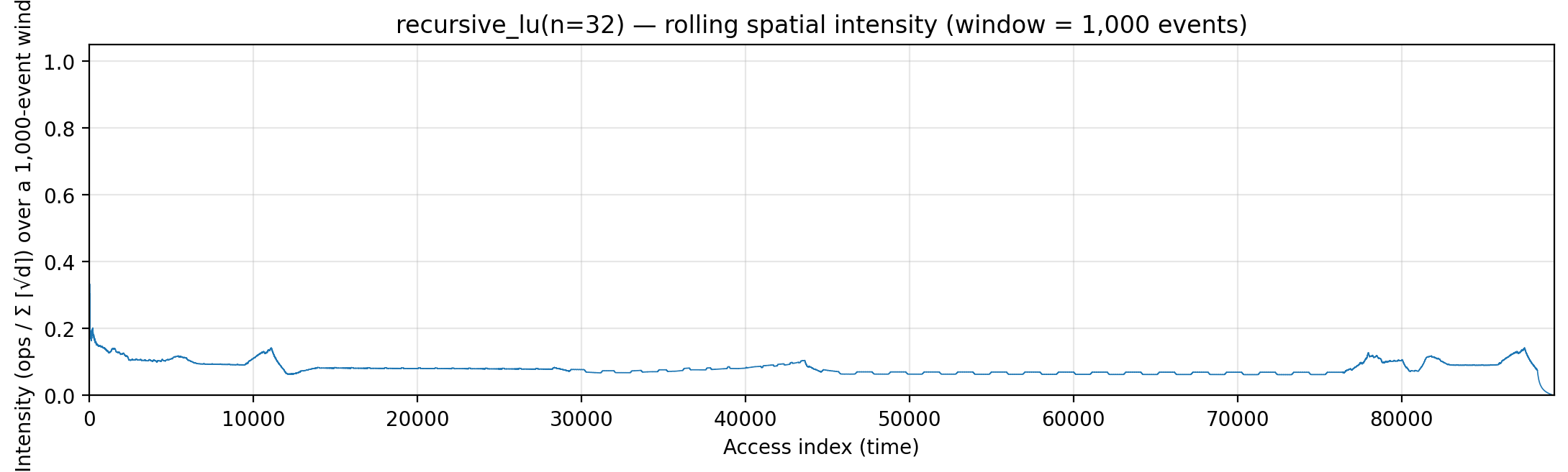
<slug>_intensity.png |
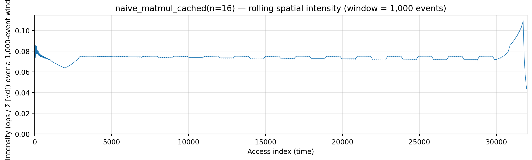
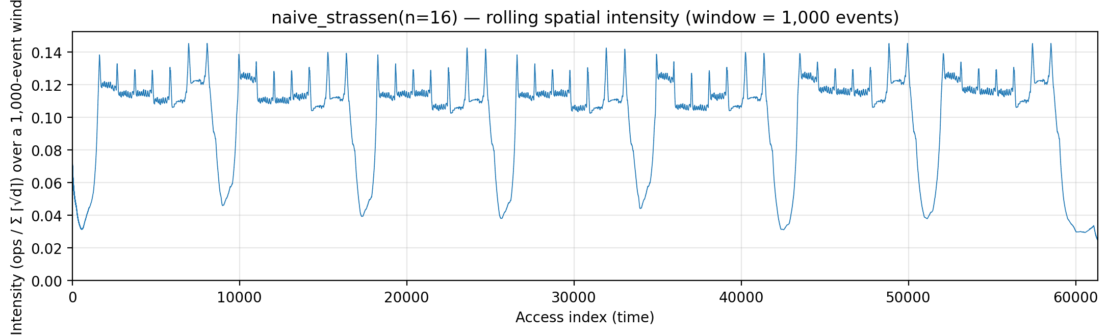
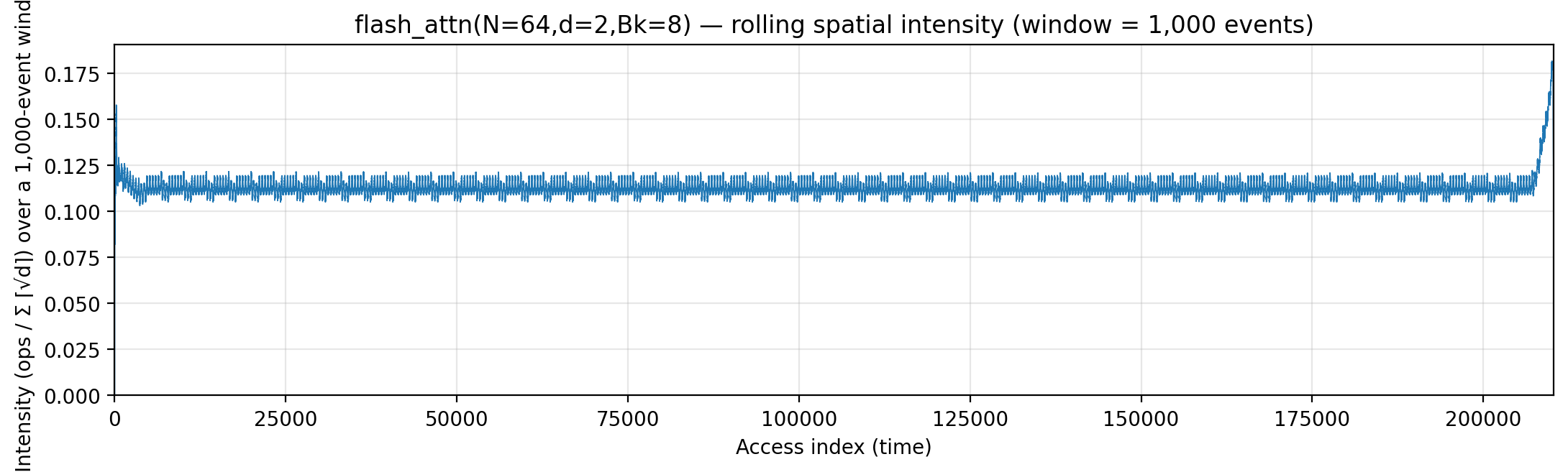
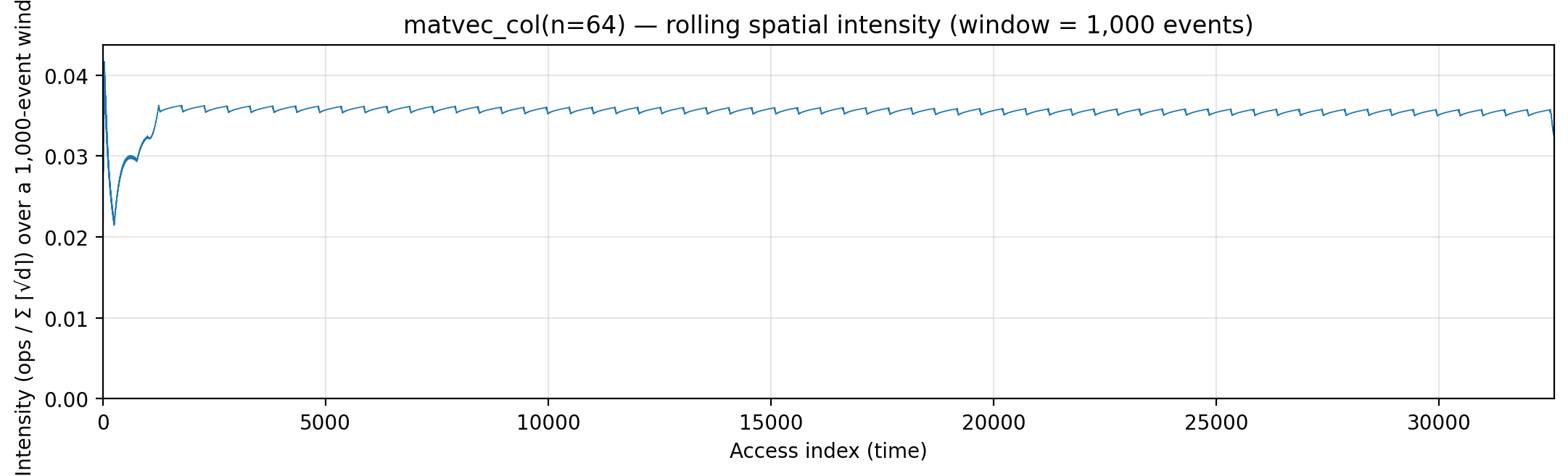
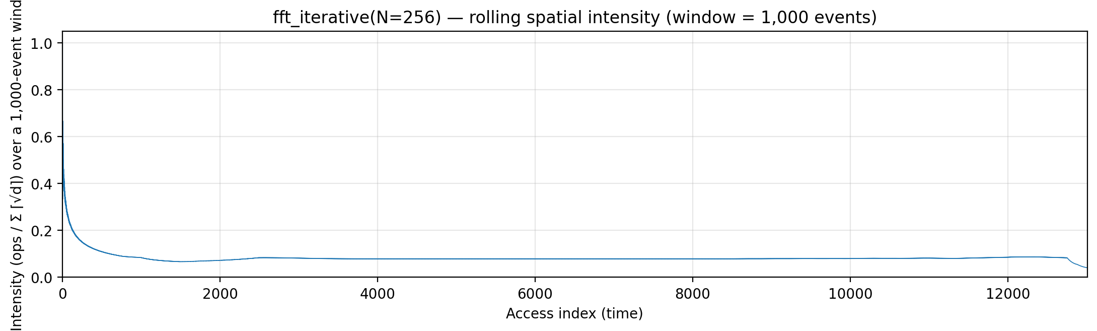
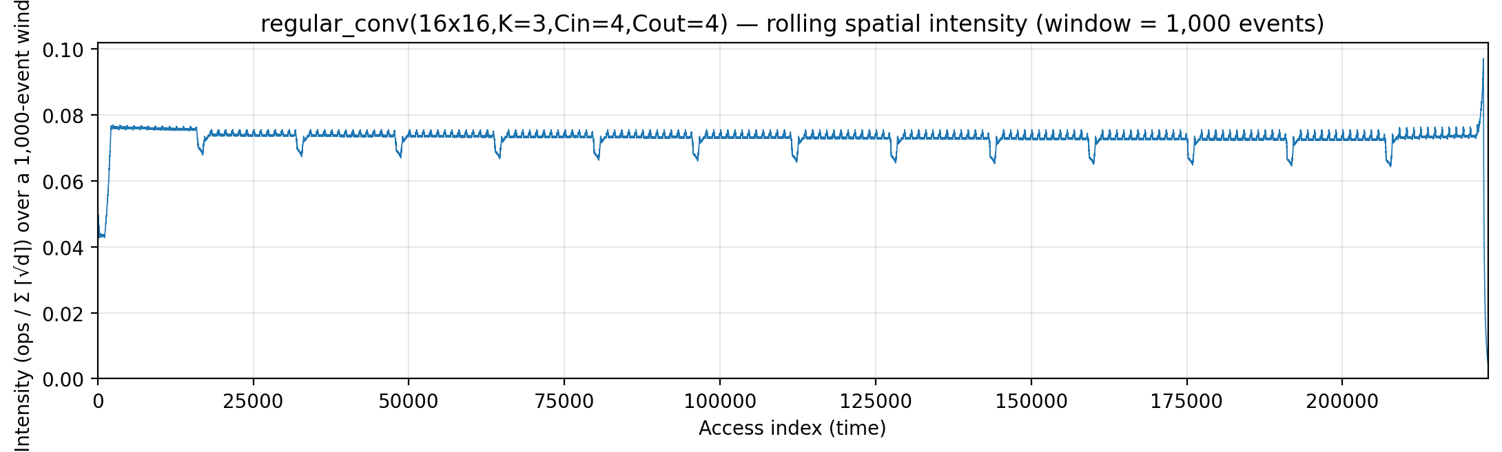
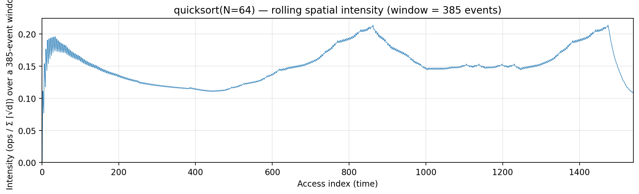
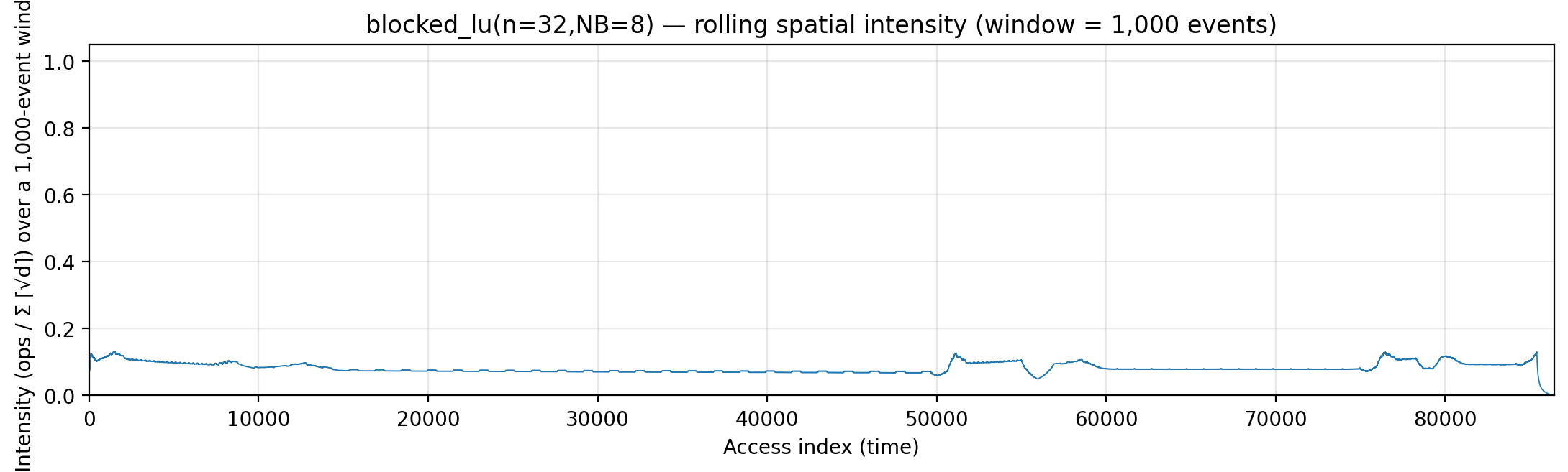
Heartbeat — rolling spatial arithmetic intensity (ops / Σ ⌈√d⌉) over a sliding window. Tiled / blocked algorithms show square-wave plateaus while a tile is in cache; naive variants stay near the floor. |
arithmetic-intensity-visualizers.md §1 |
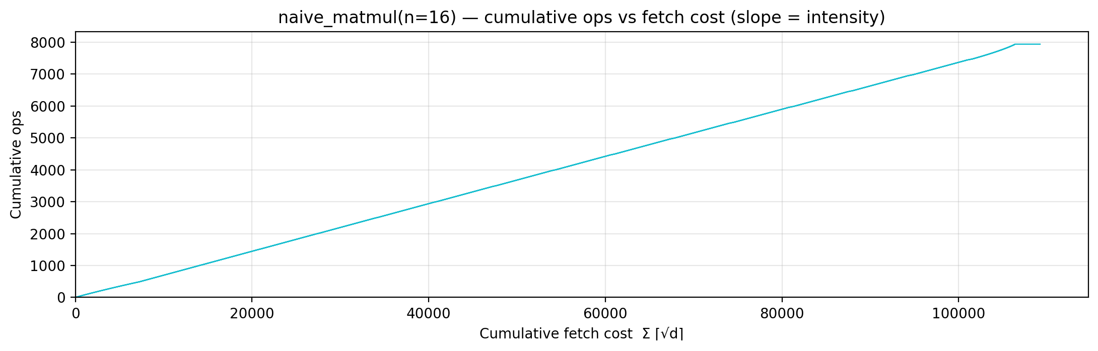
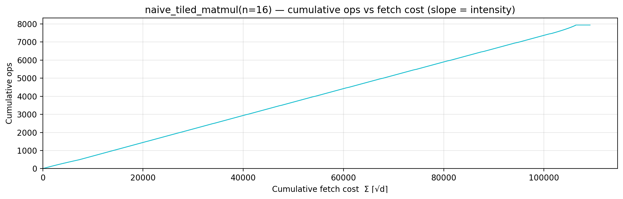
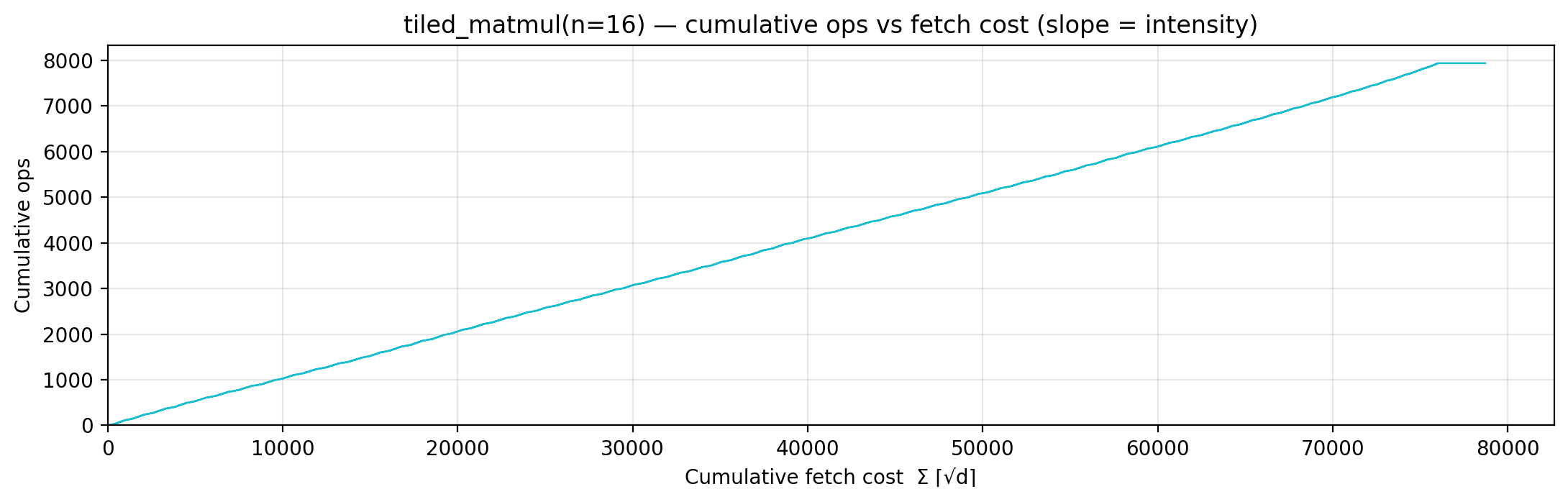
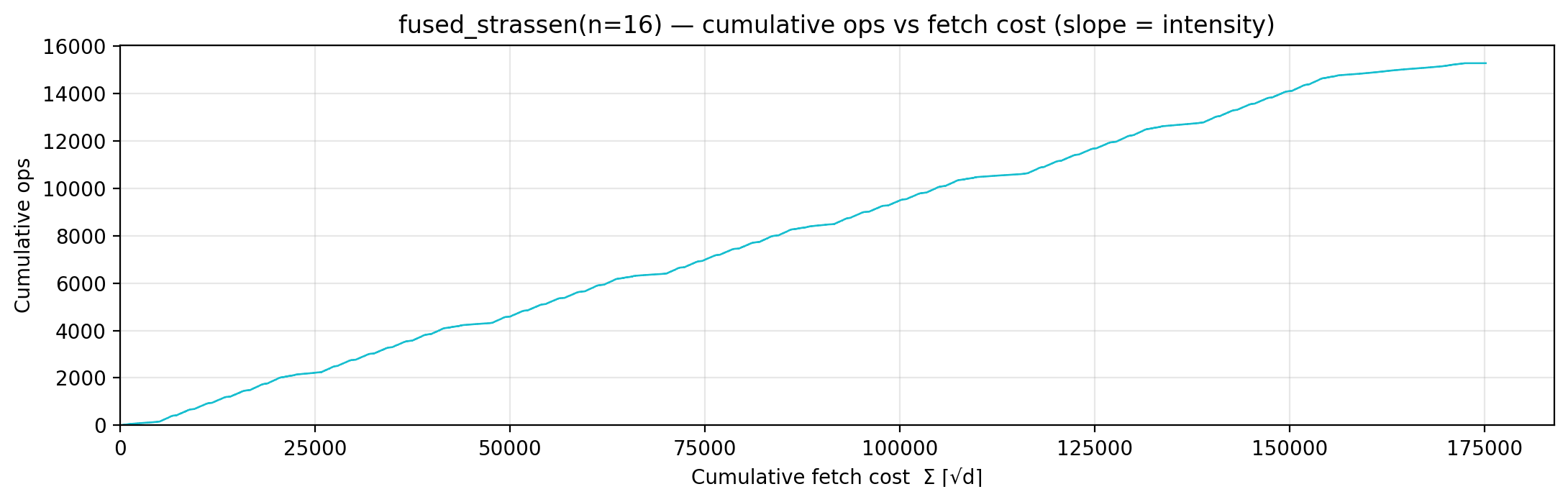
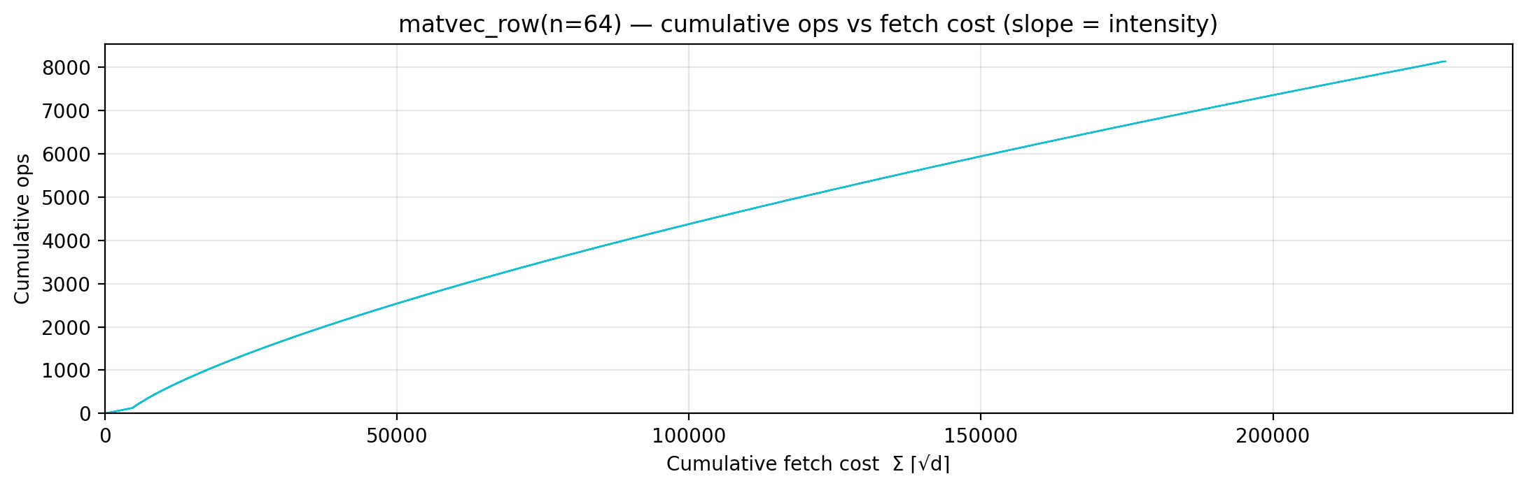
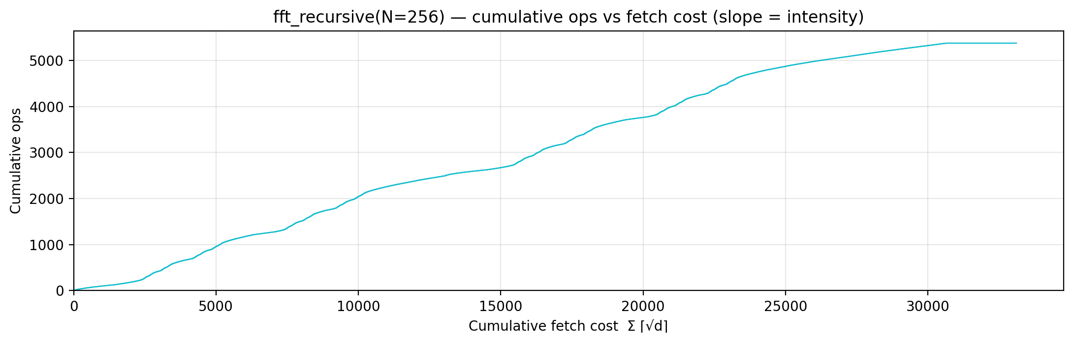
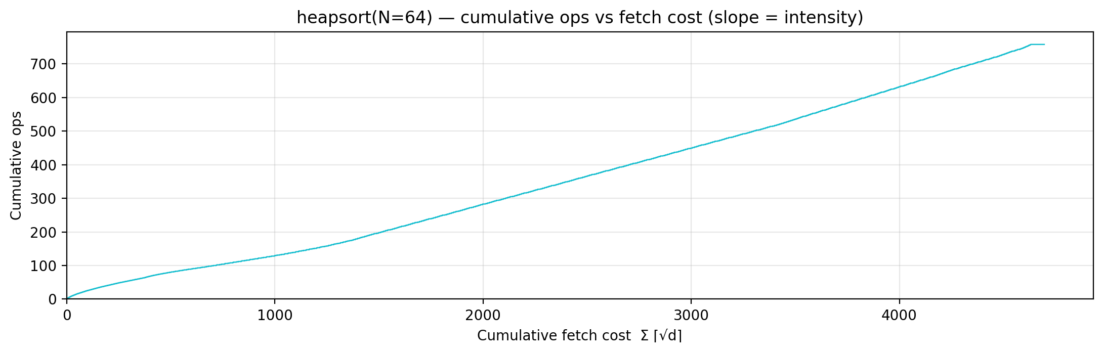
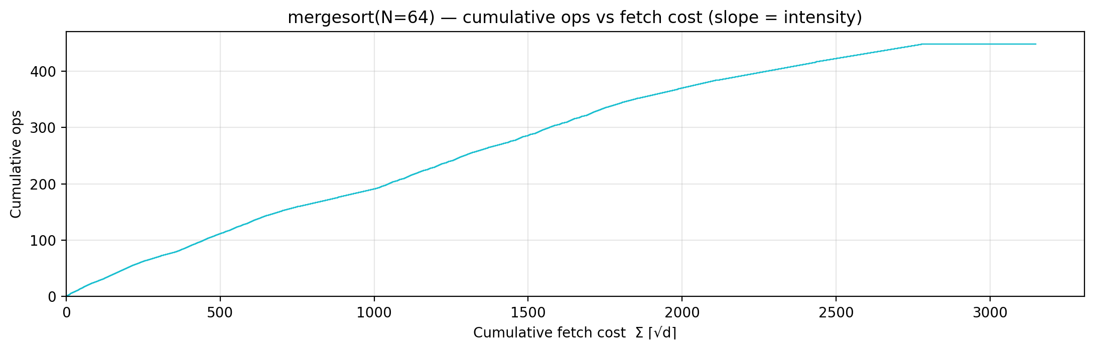
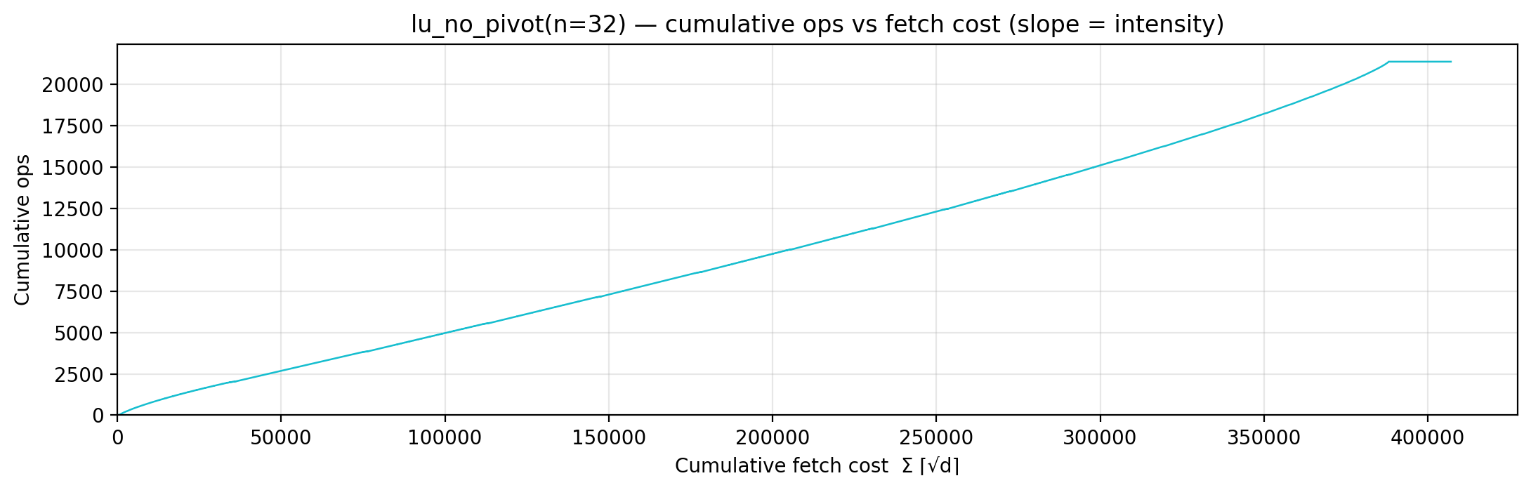
<slug>_phase_diagram.png |
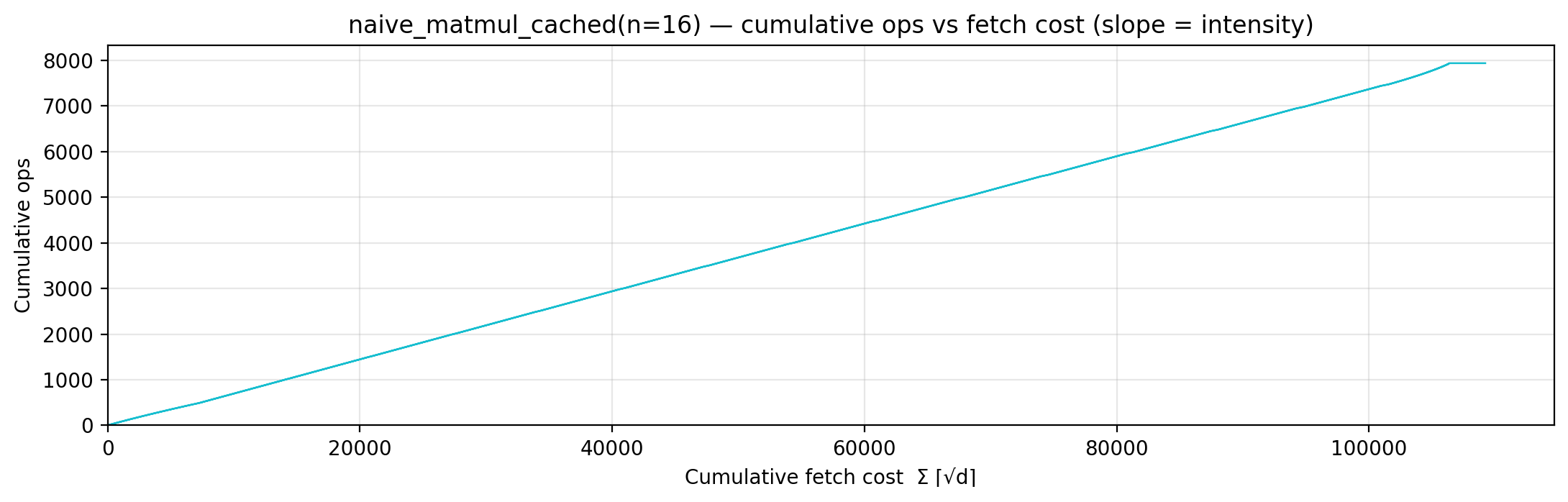
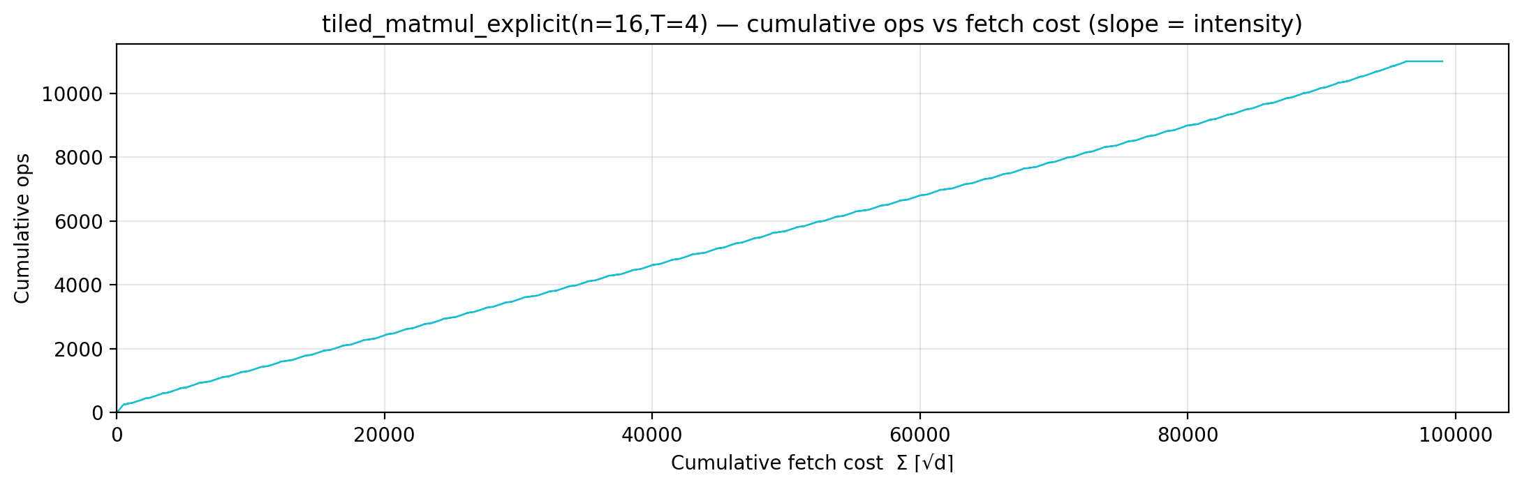
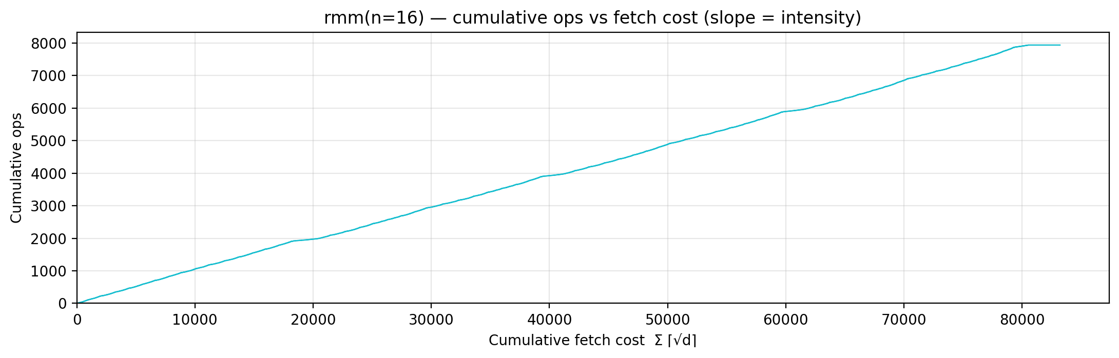
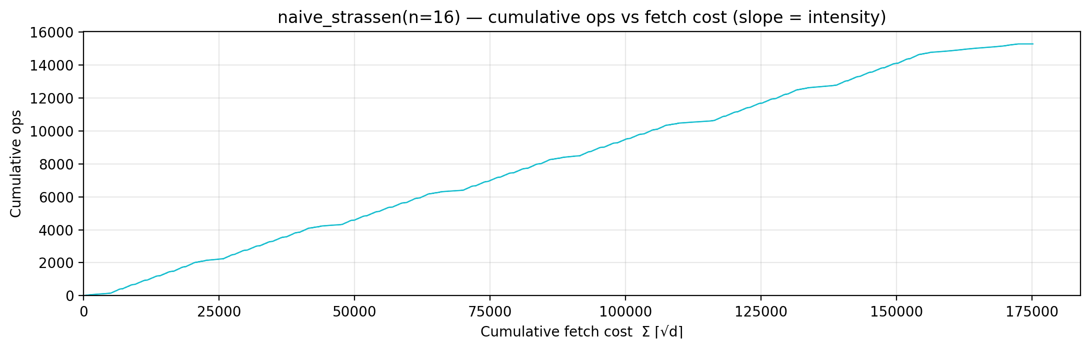
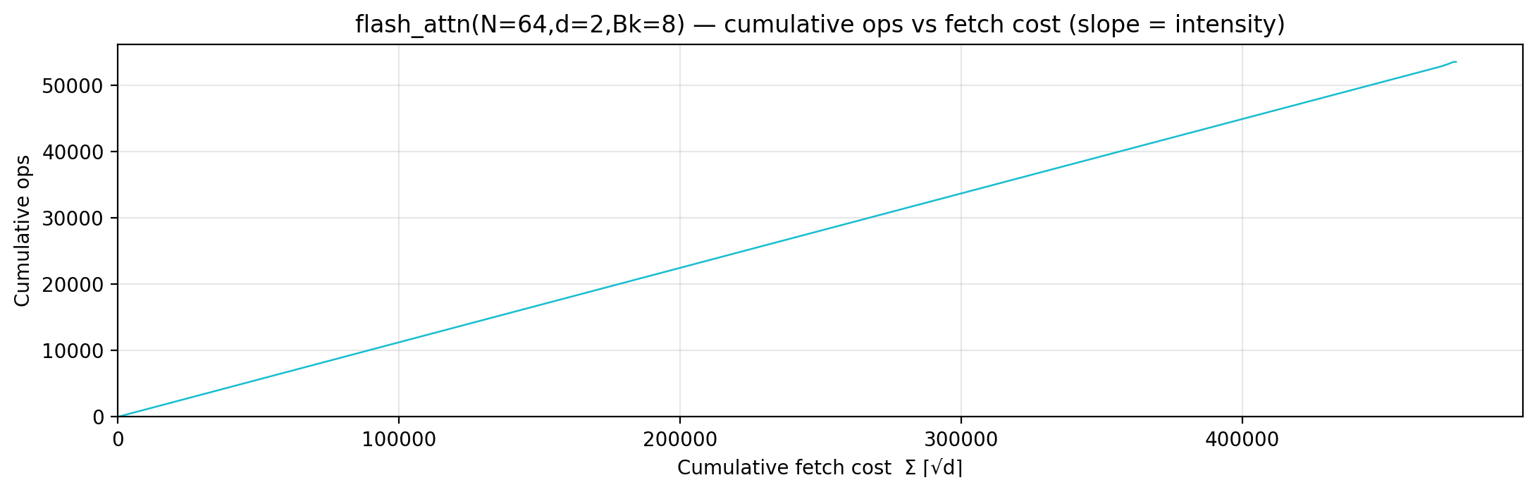
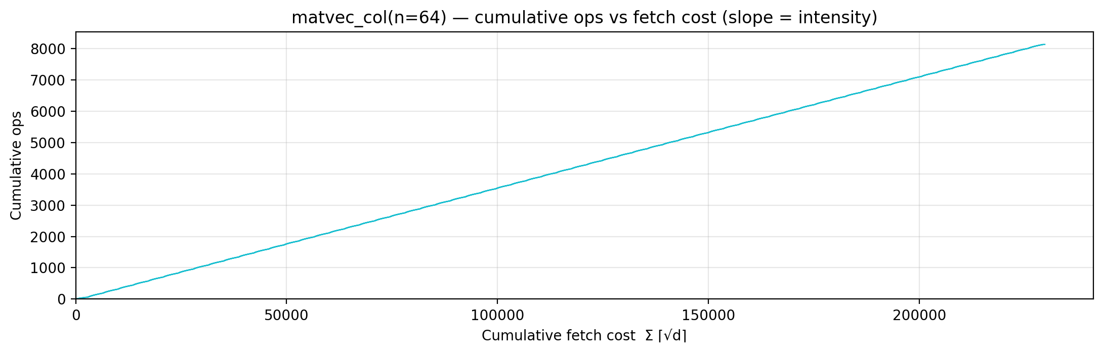
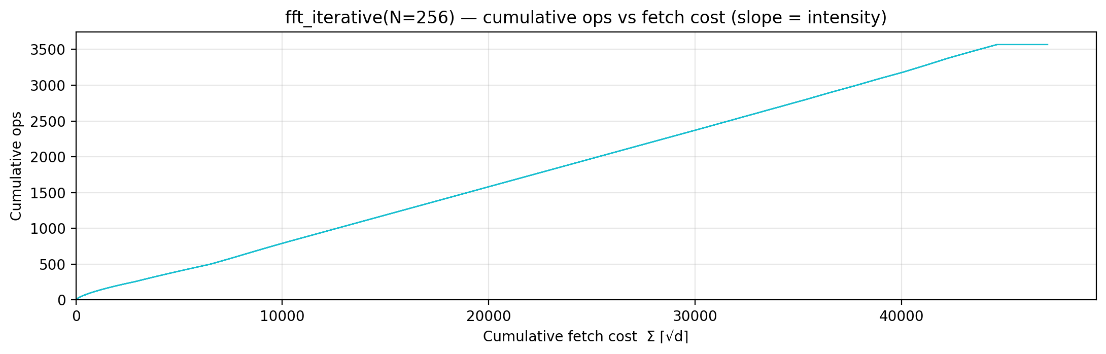
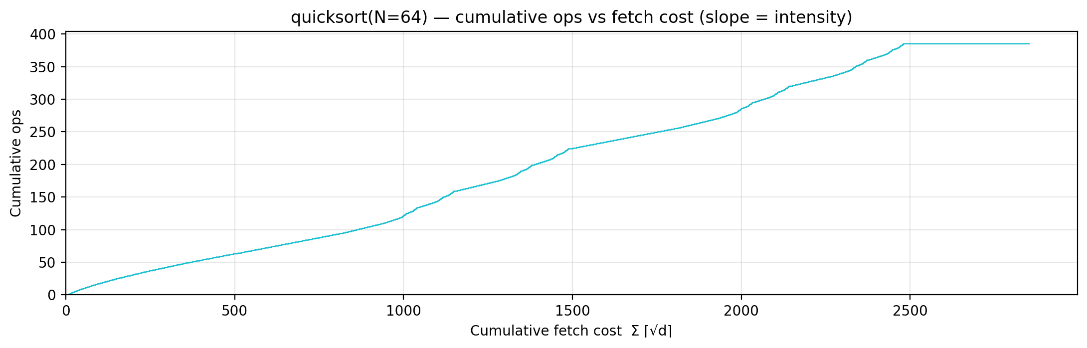
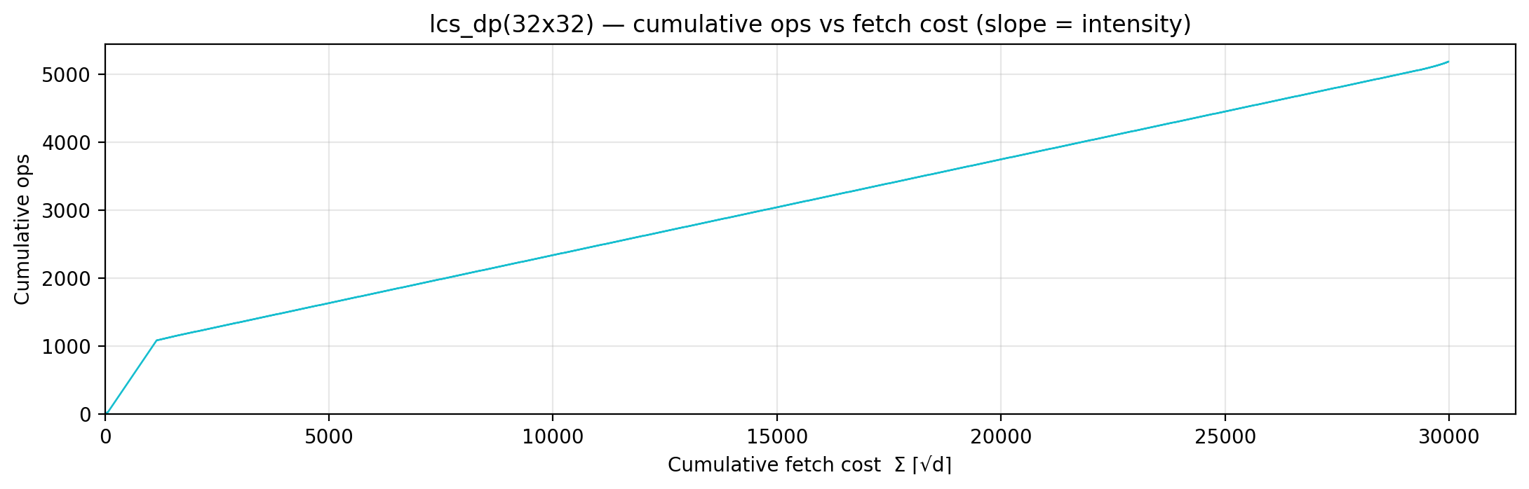
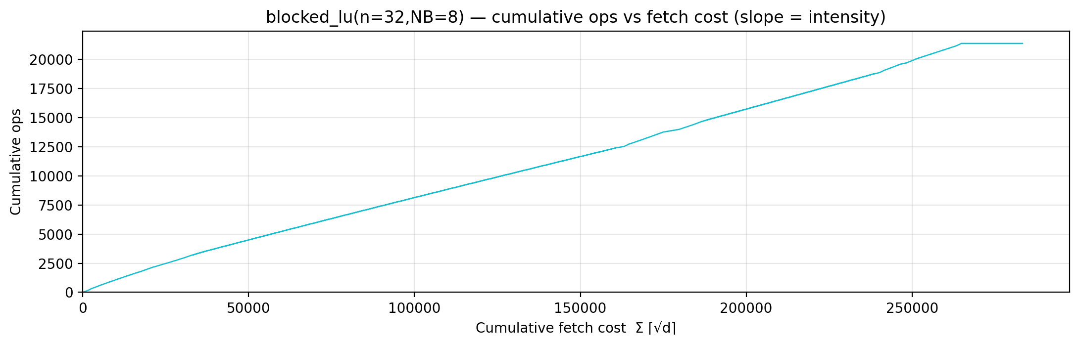
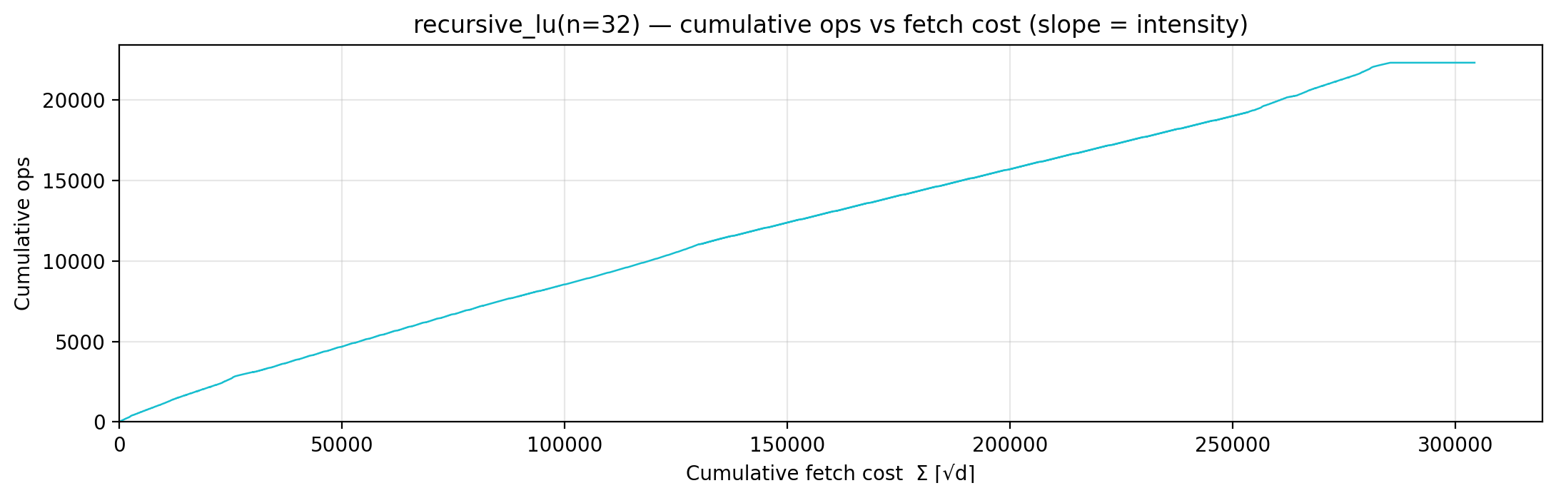
Spatial Phase Diagram — cumulative ops (y) vs cumulative fetch cost (x). The line slope = instantaneous intensity; tiled algorithms trace a steep staircase, naive ones a shallow diagonal. | arithmetic-intensity-visualizers.md §2 |
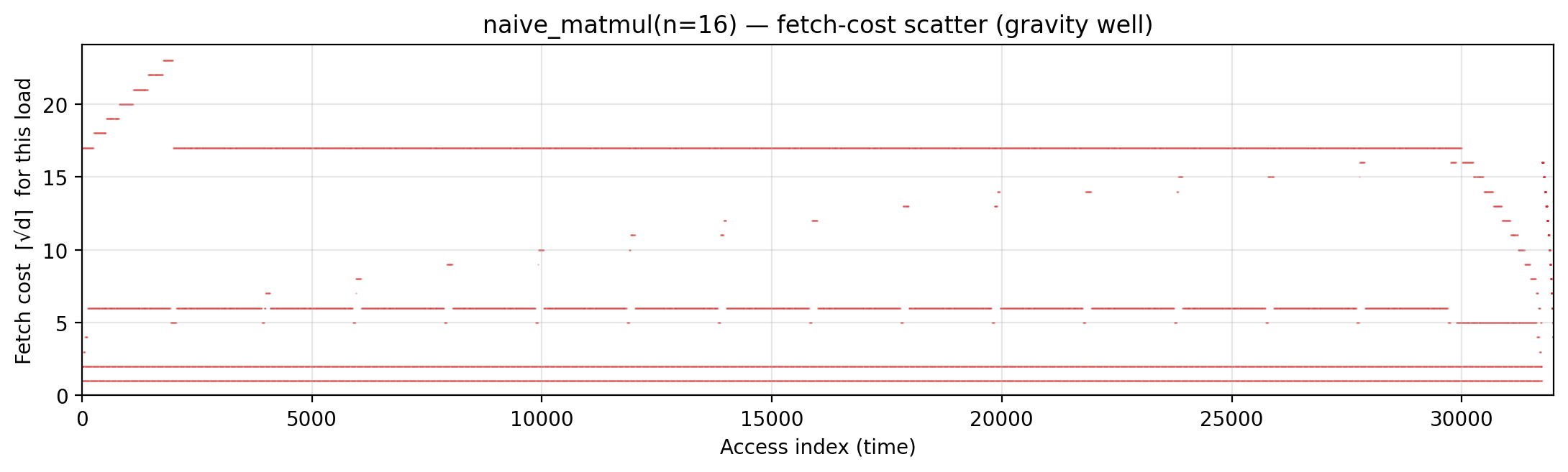
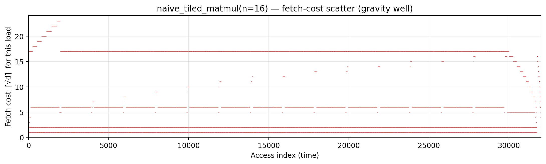
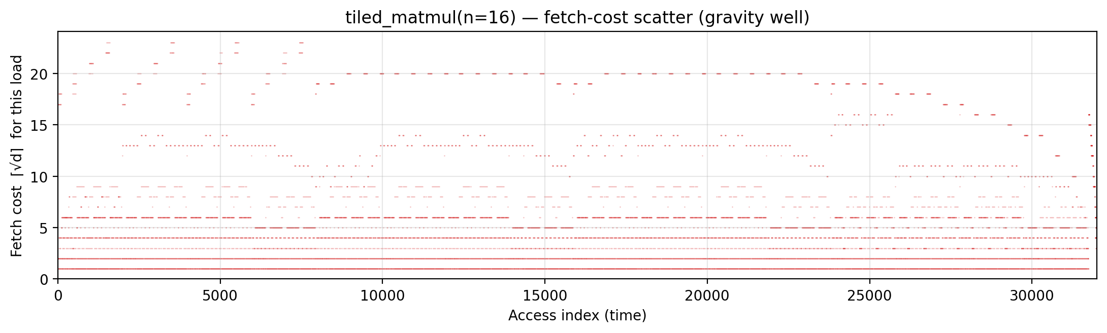
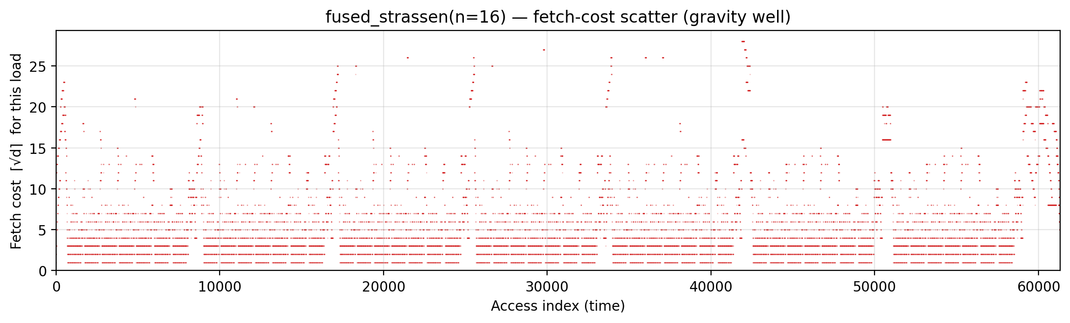
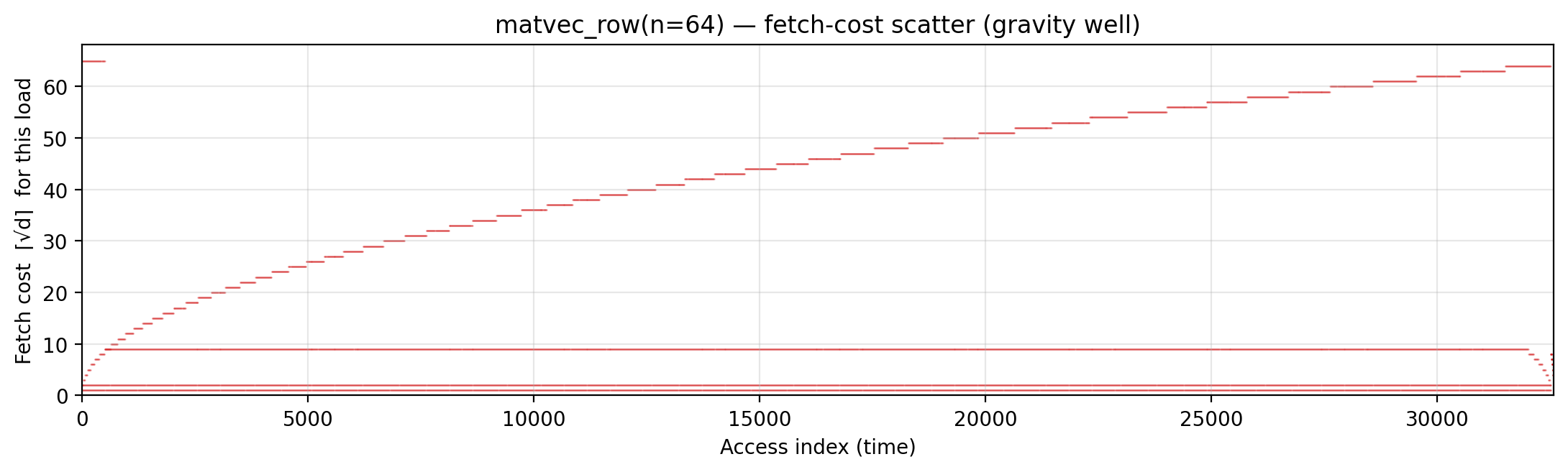
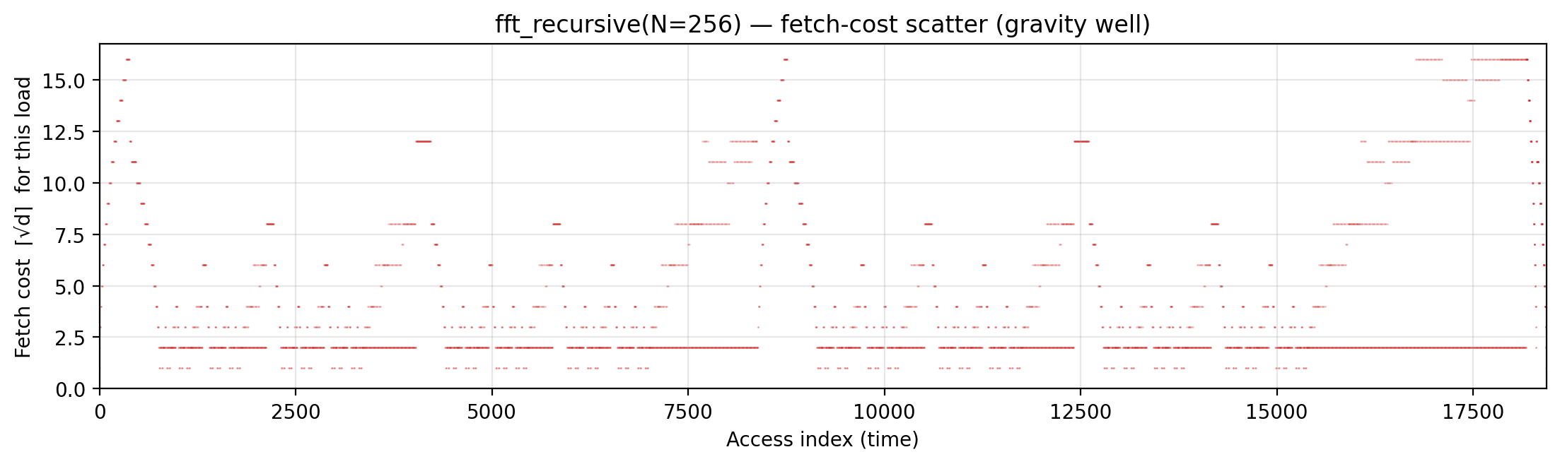
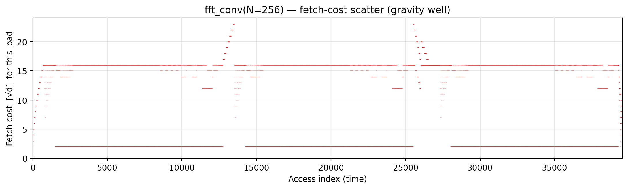
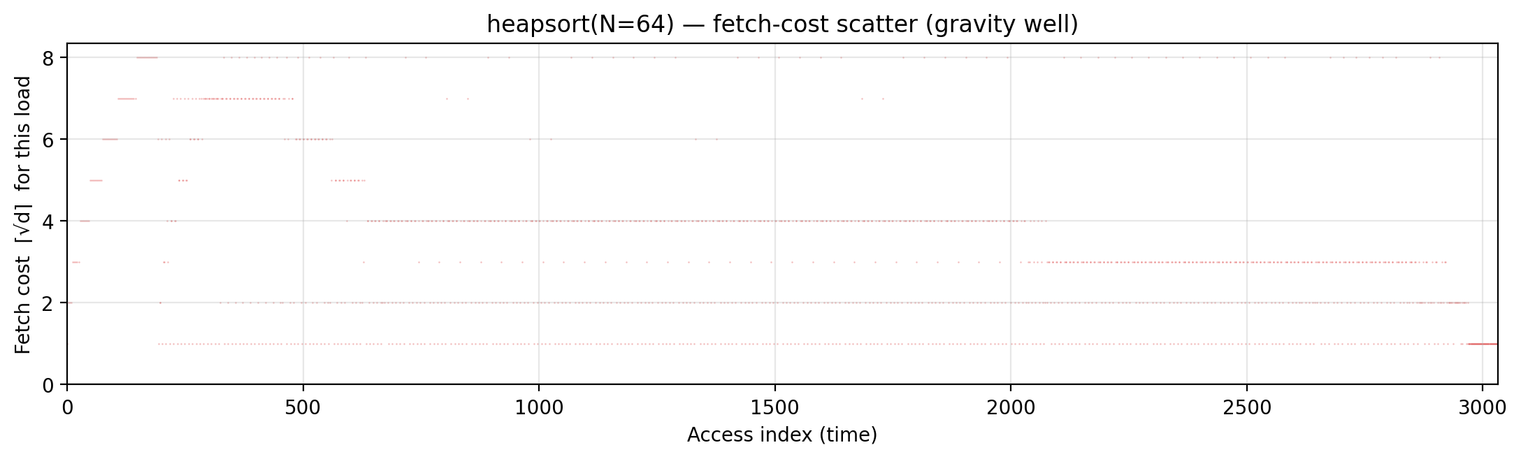
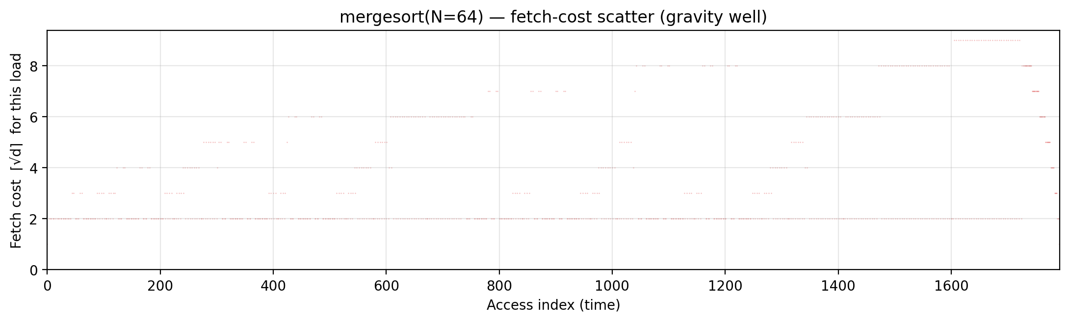
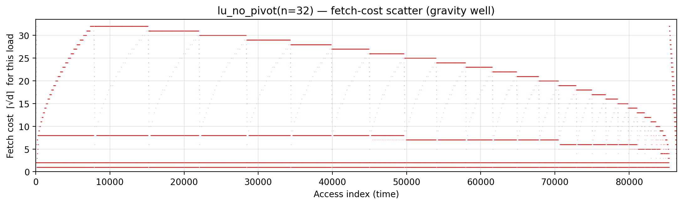
<slug>_gravity_well.png |
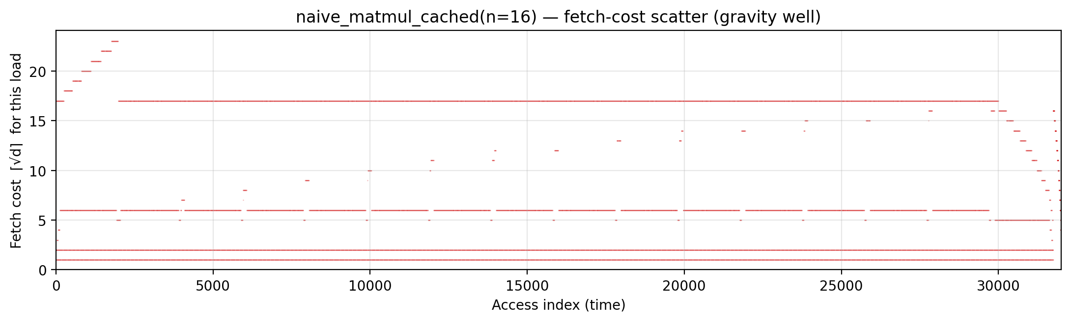
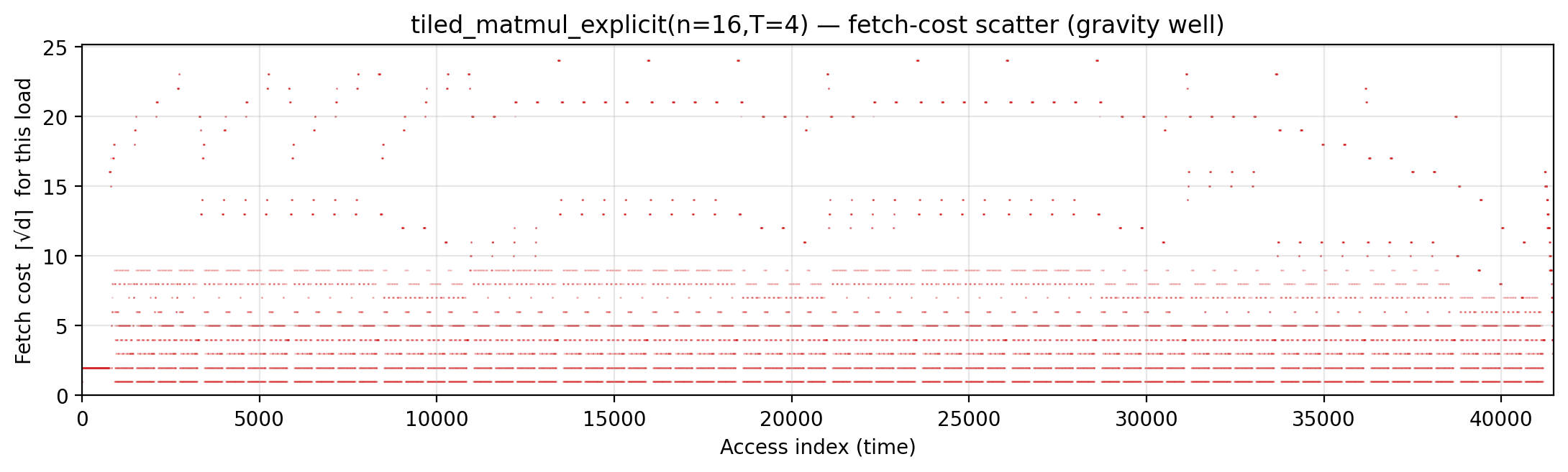
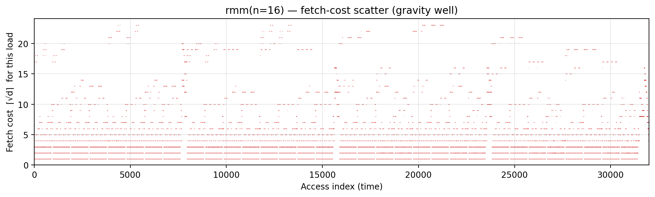
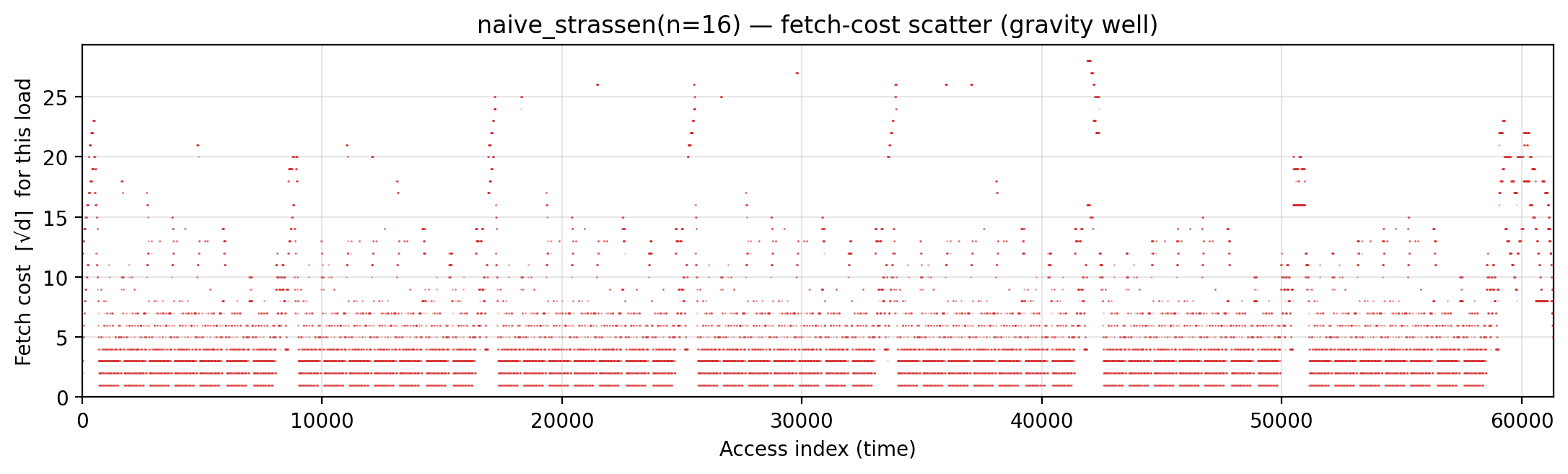
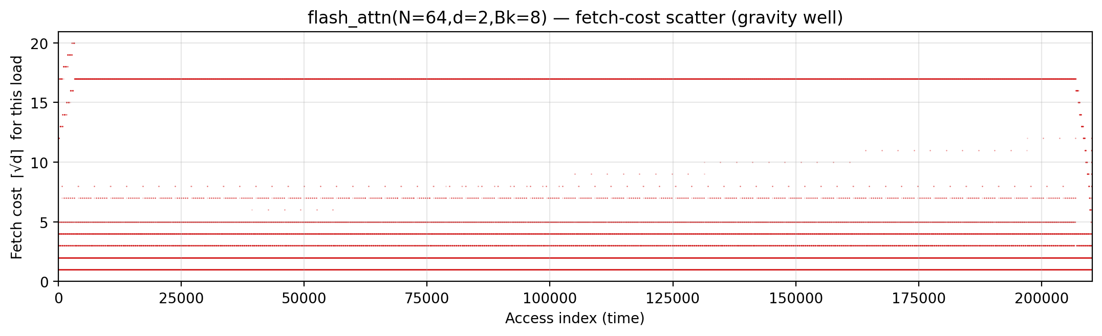
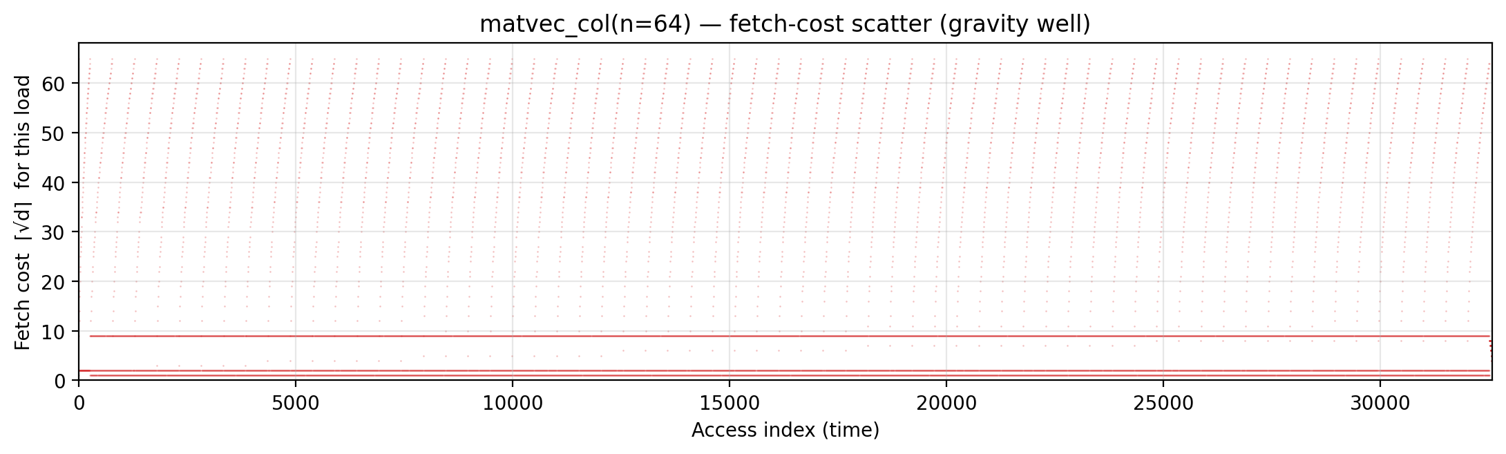
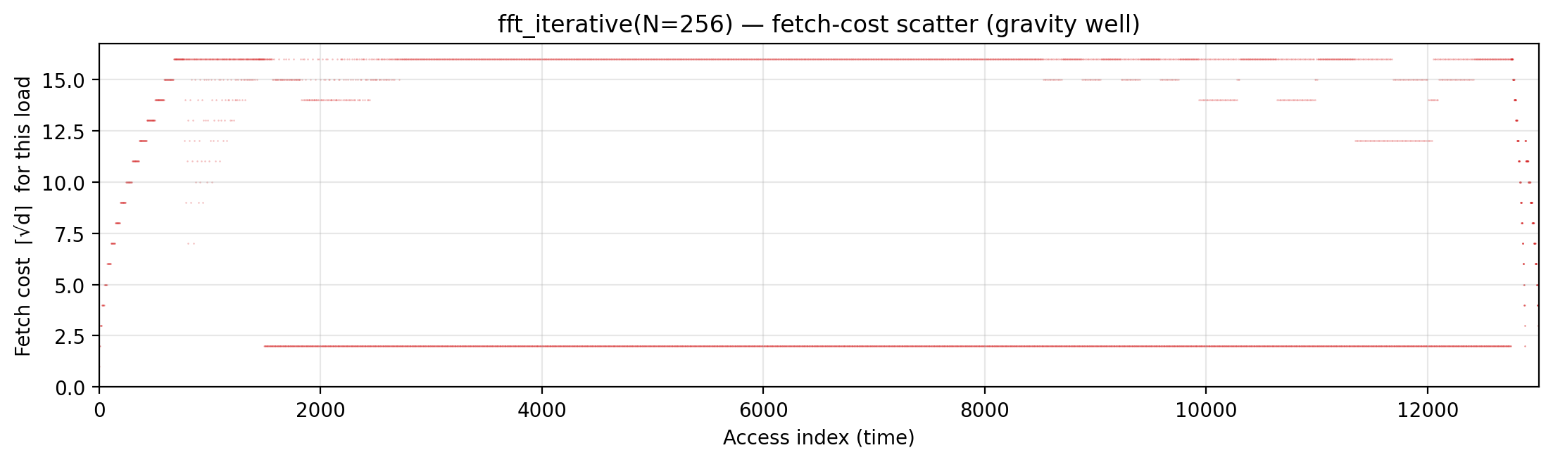
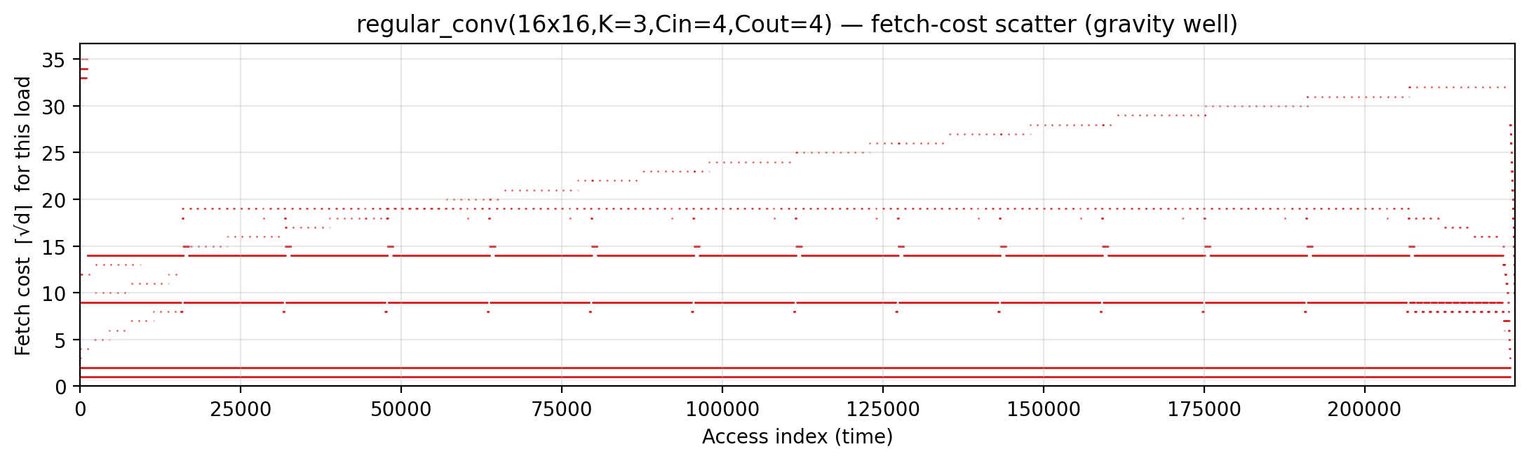
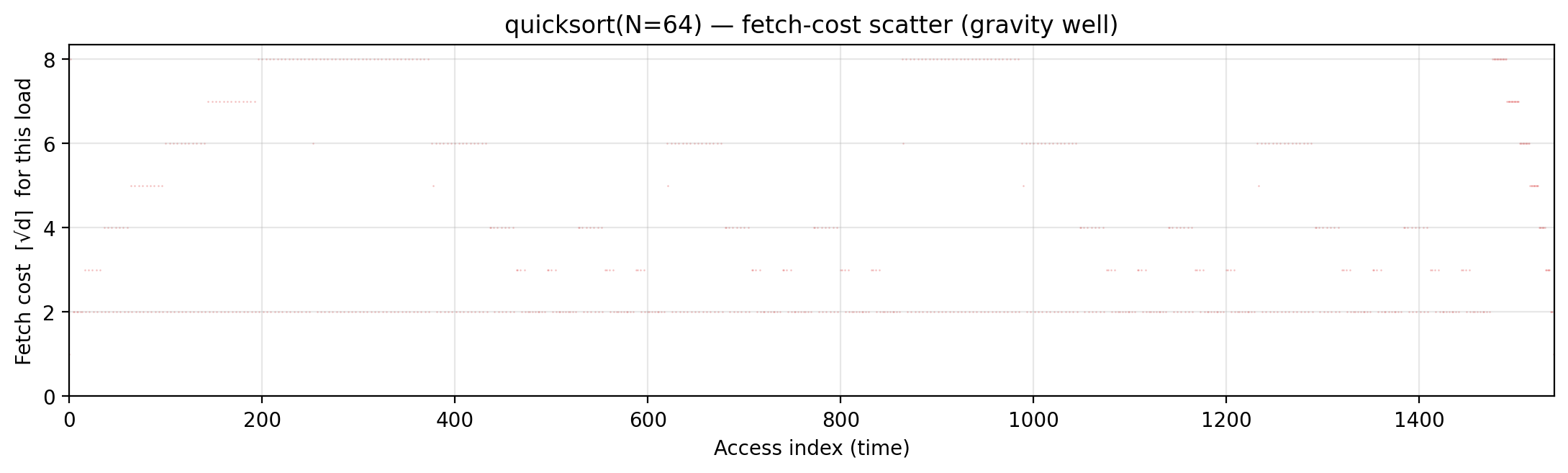
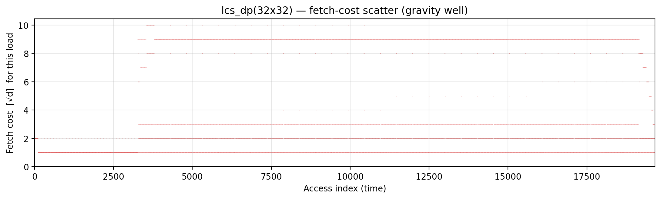
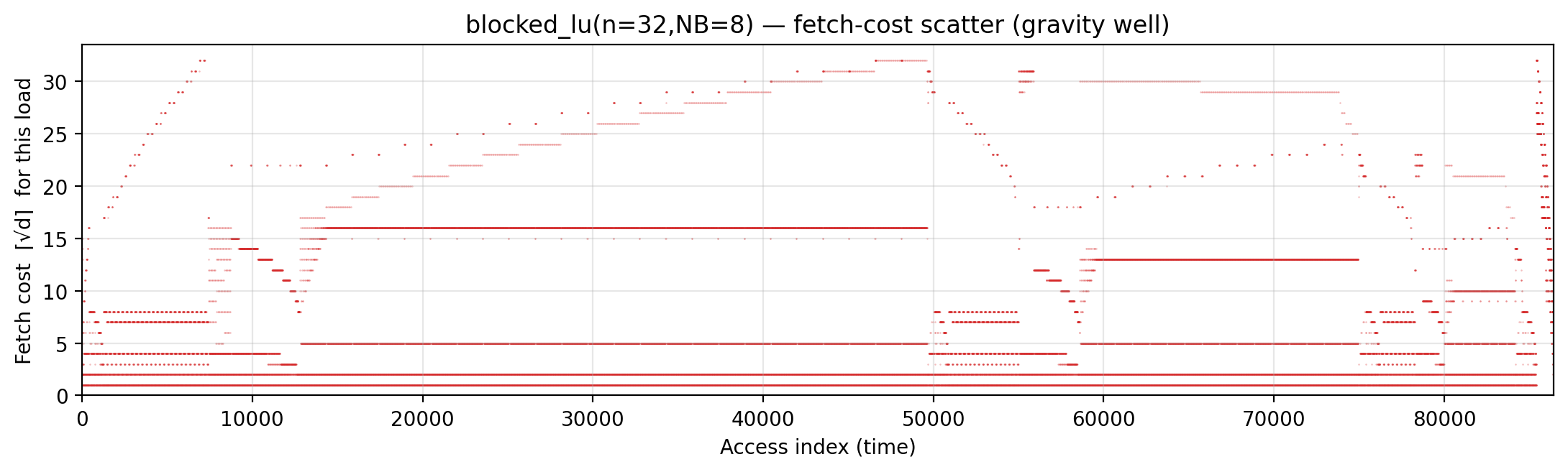
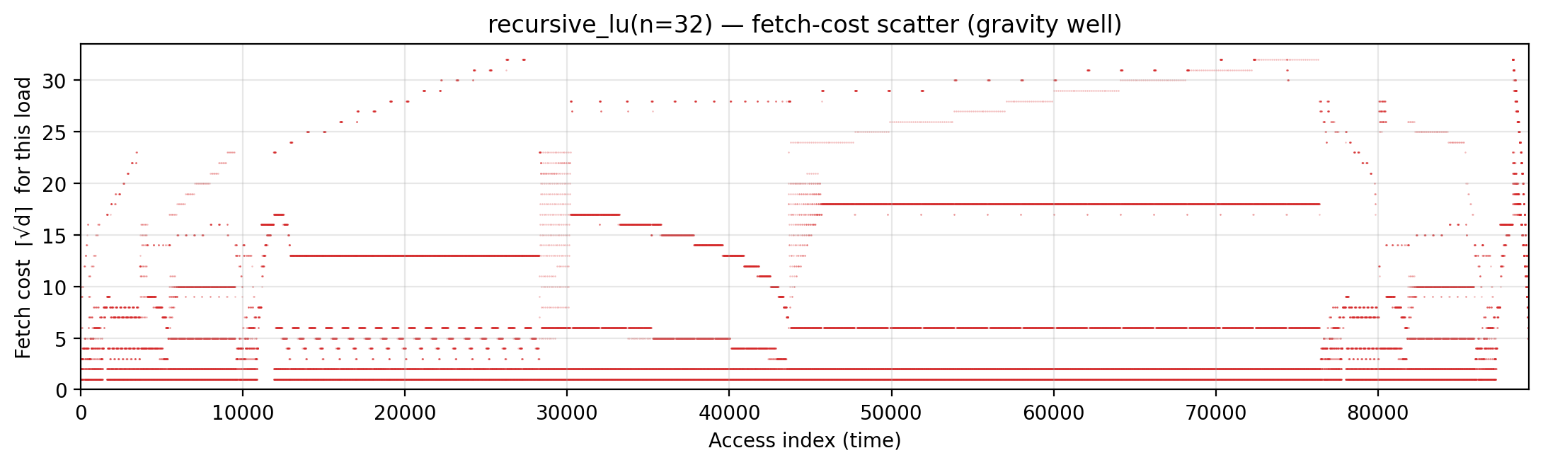
Gravity Well — per-load fetch-cost ⌈√d⌉ scatter. Dense low bands = tight orbital footprint (most reads near the ALU); high spray = excursions into deep memory. |
arithmetic-intensity-visualizers.md §3 |
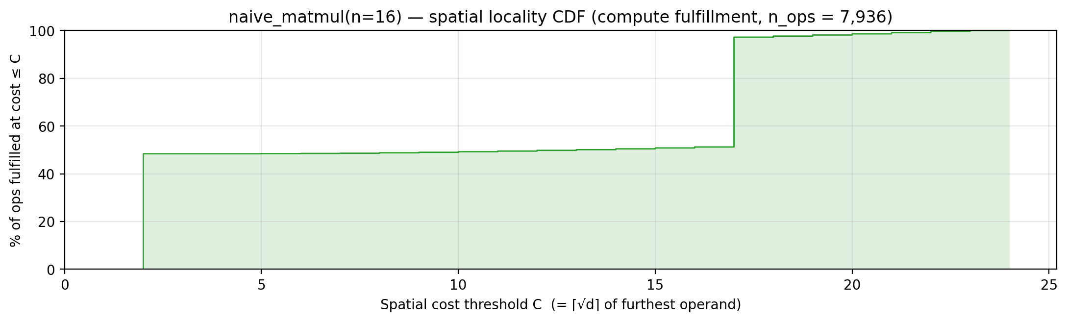
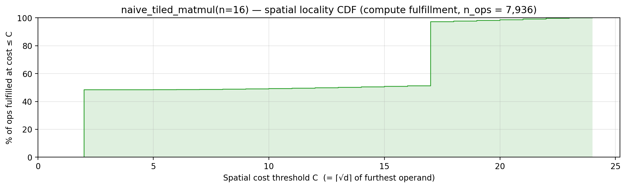
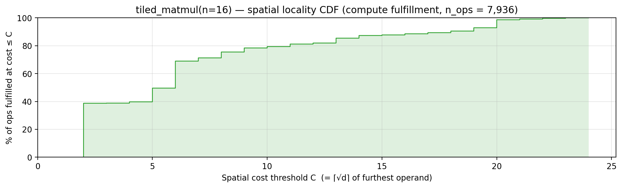
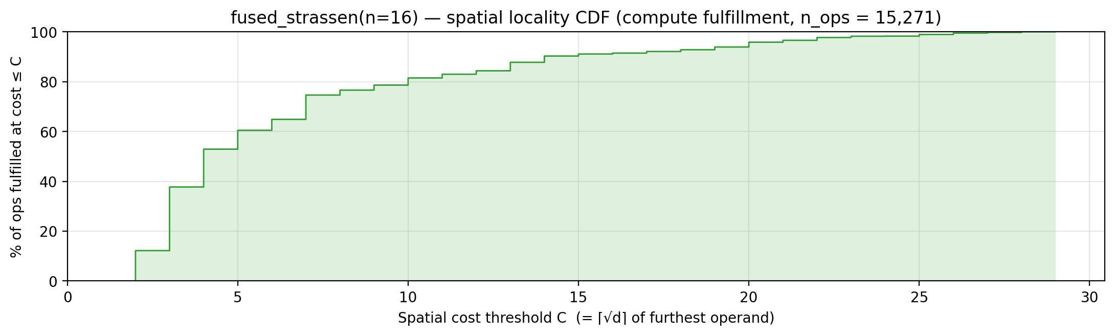
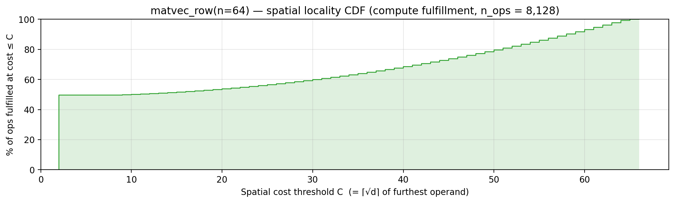
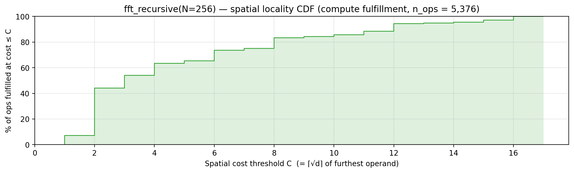
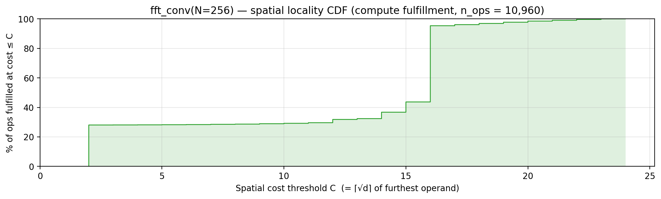
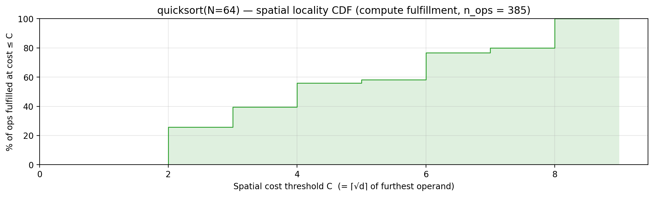
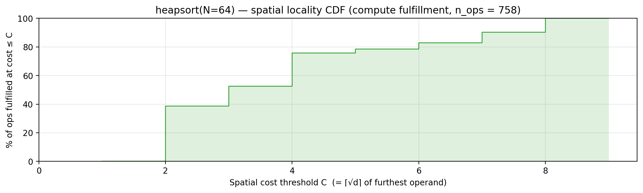
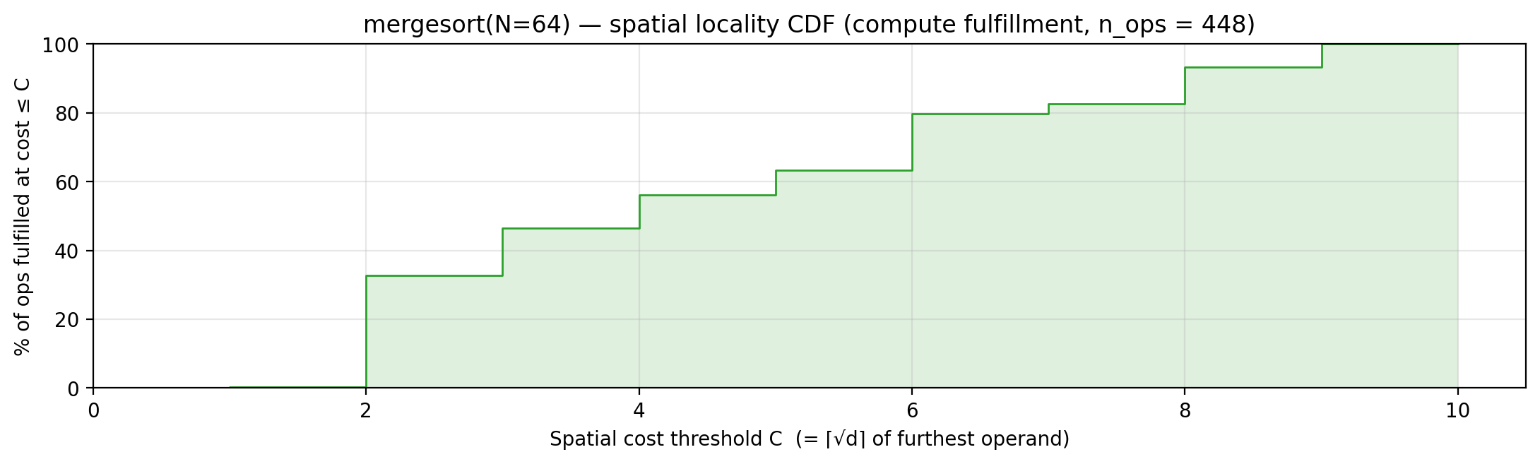
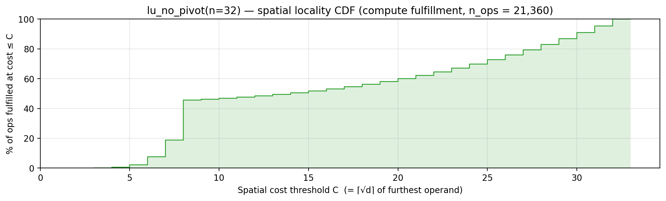
<slug>_locality_cdf.png |
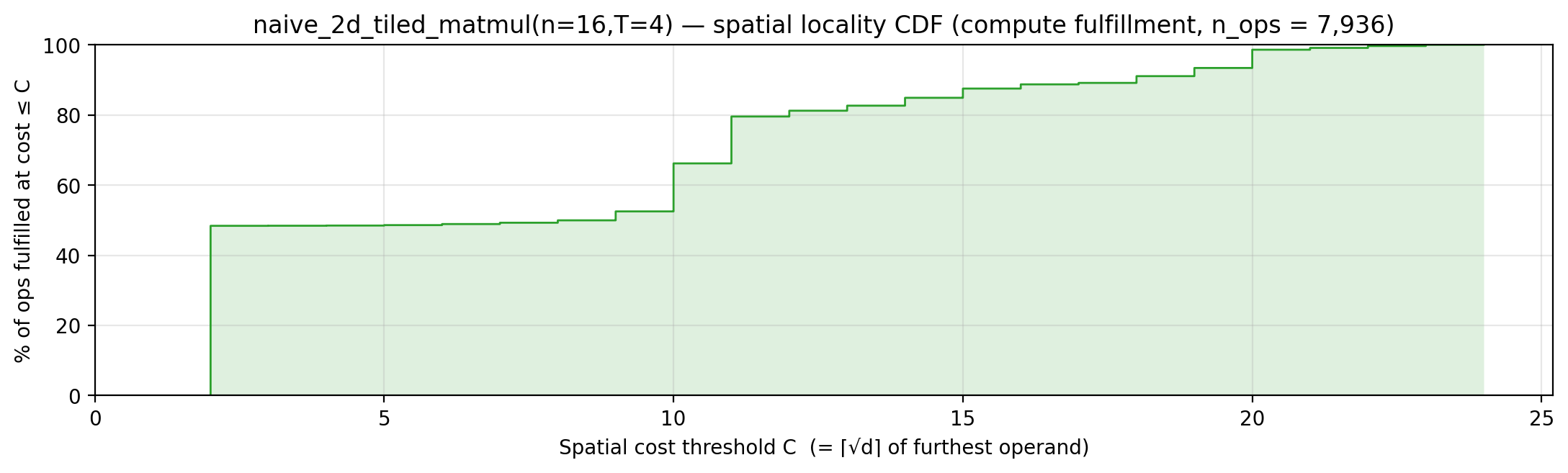
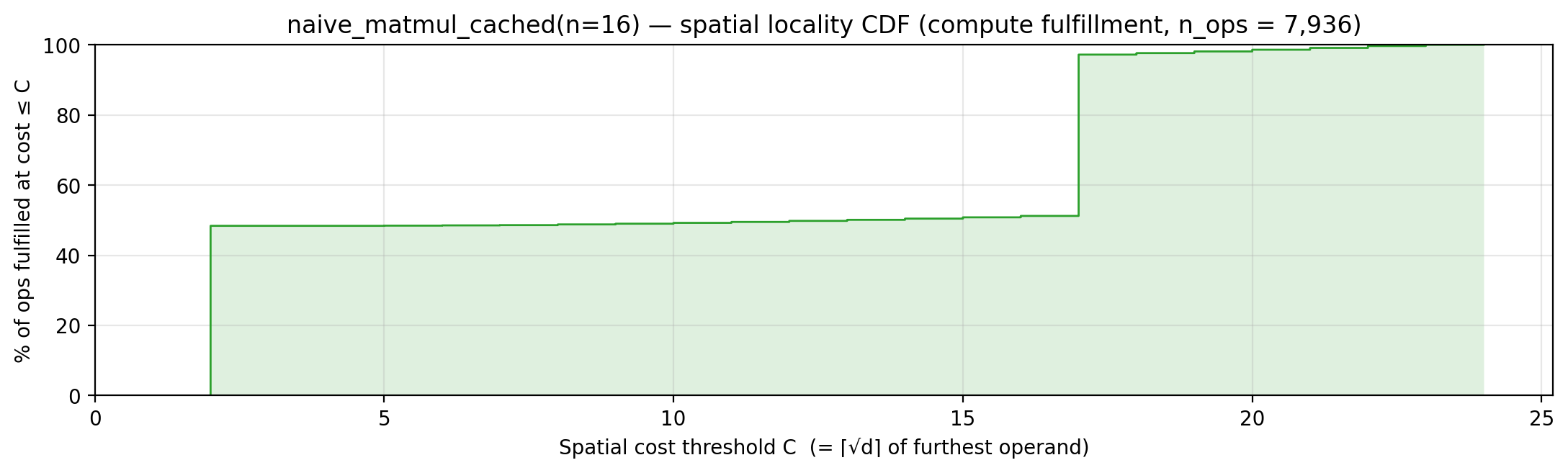
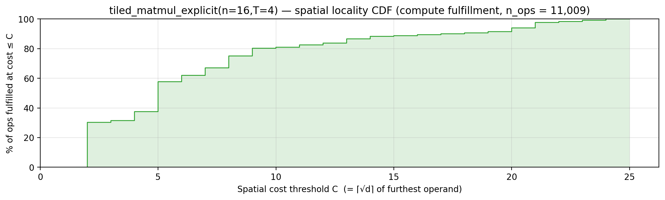
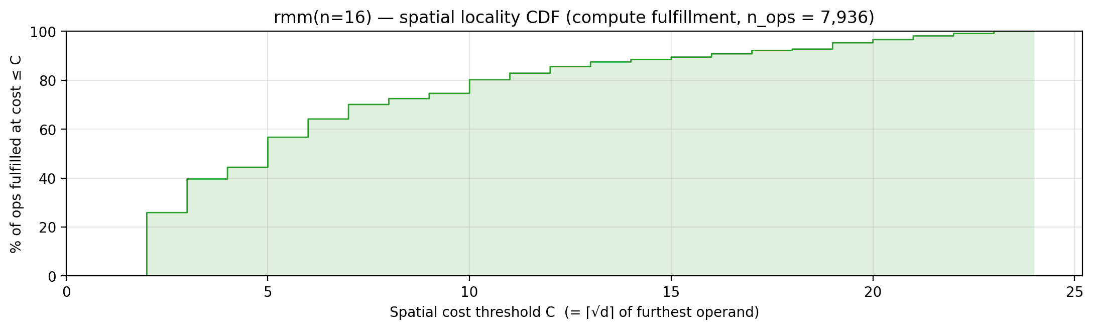
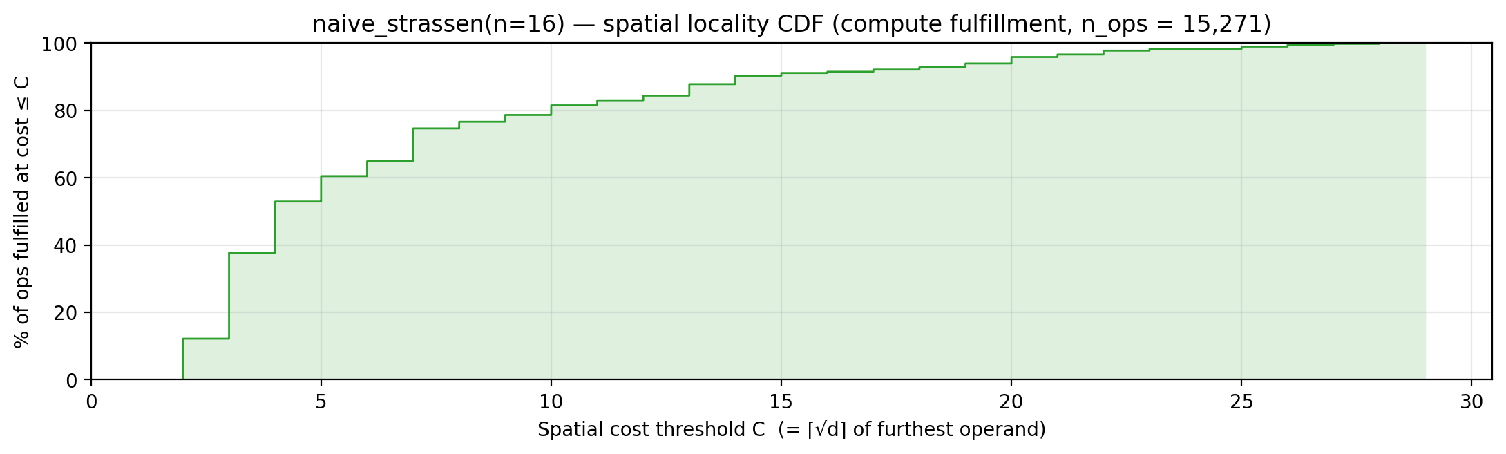
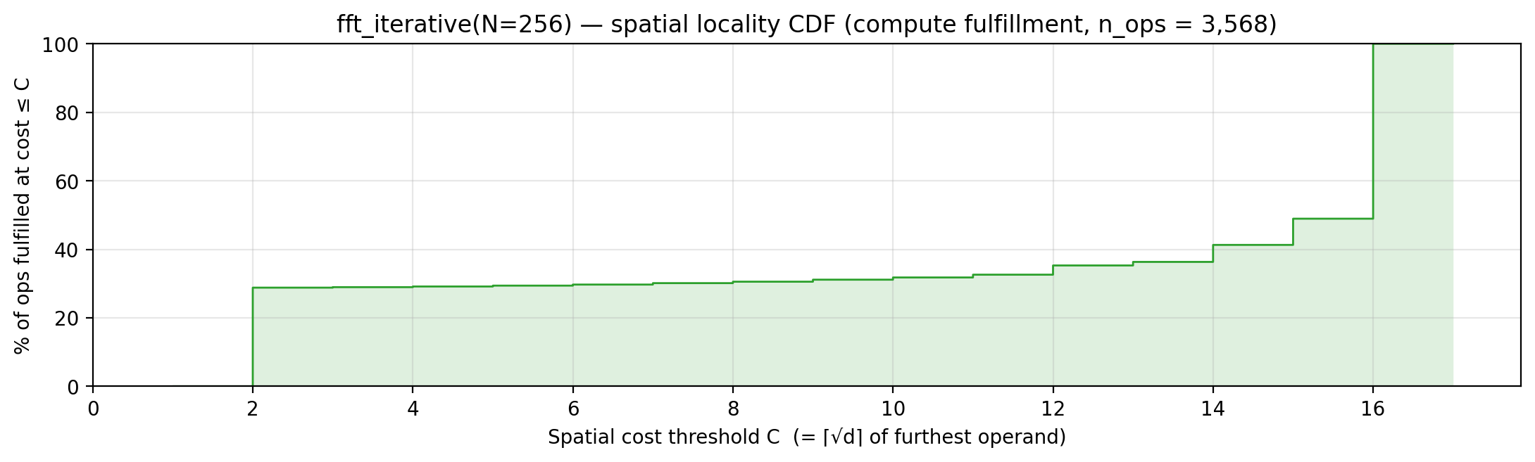
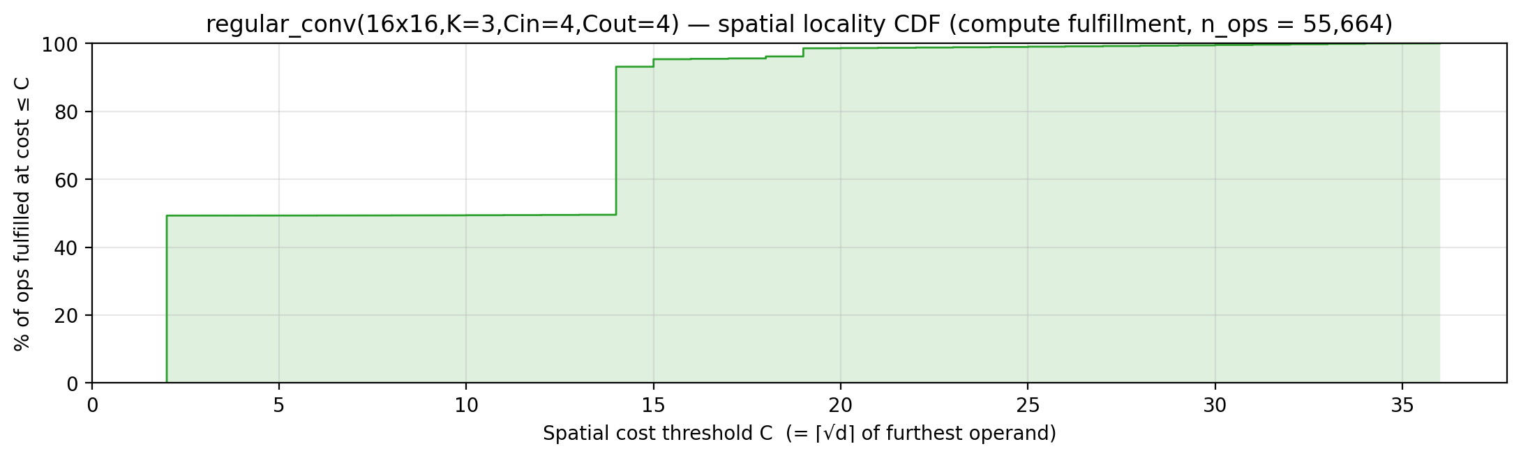
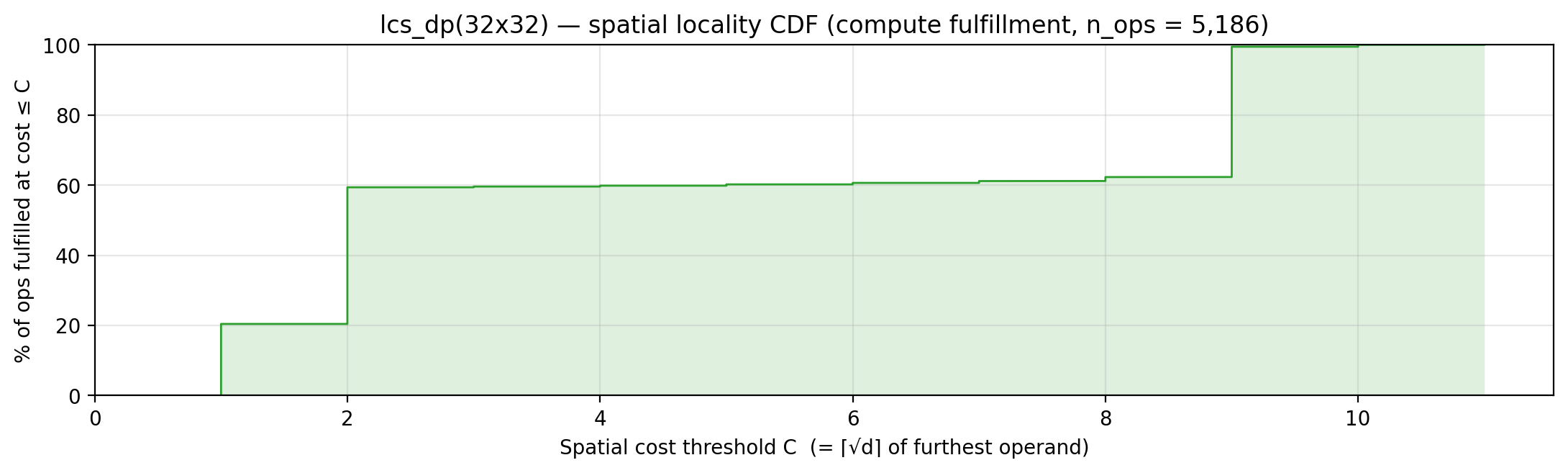
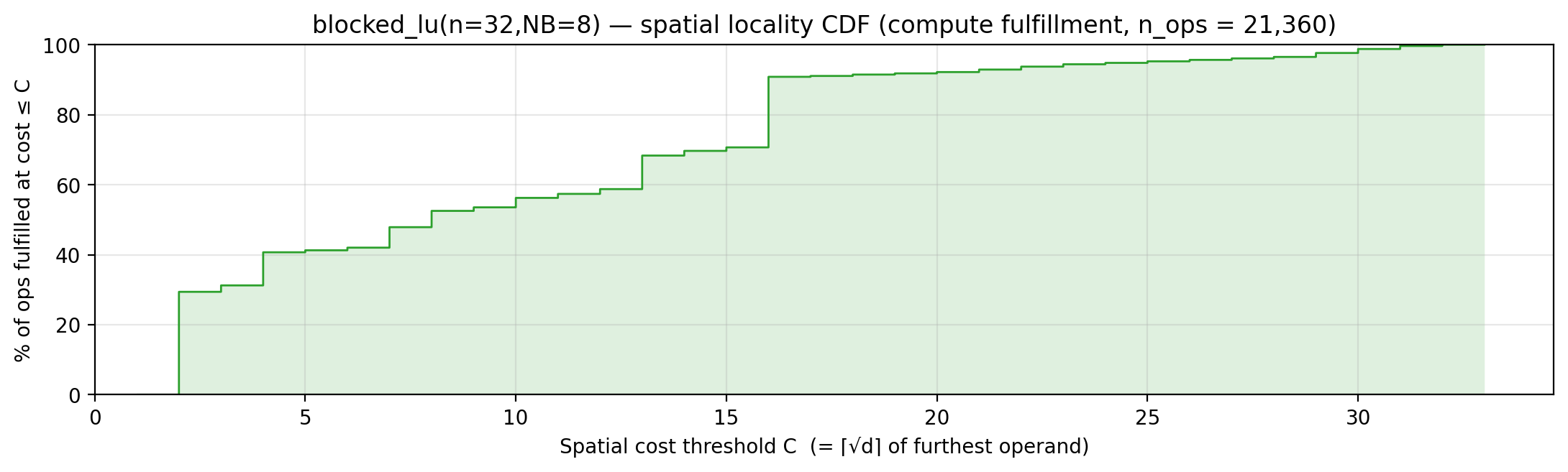
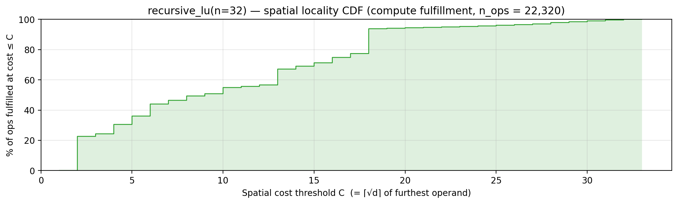
Compute-Fulfillment CDF — % of arithmetic ops whose furthest-fetched operand cost ≤ C, for each radius C. A sheer cliff face near the origin means the algorithm’s working volume is quarantined close to the ALU. | arithmetic-intensity-visualizers.md §4 |
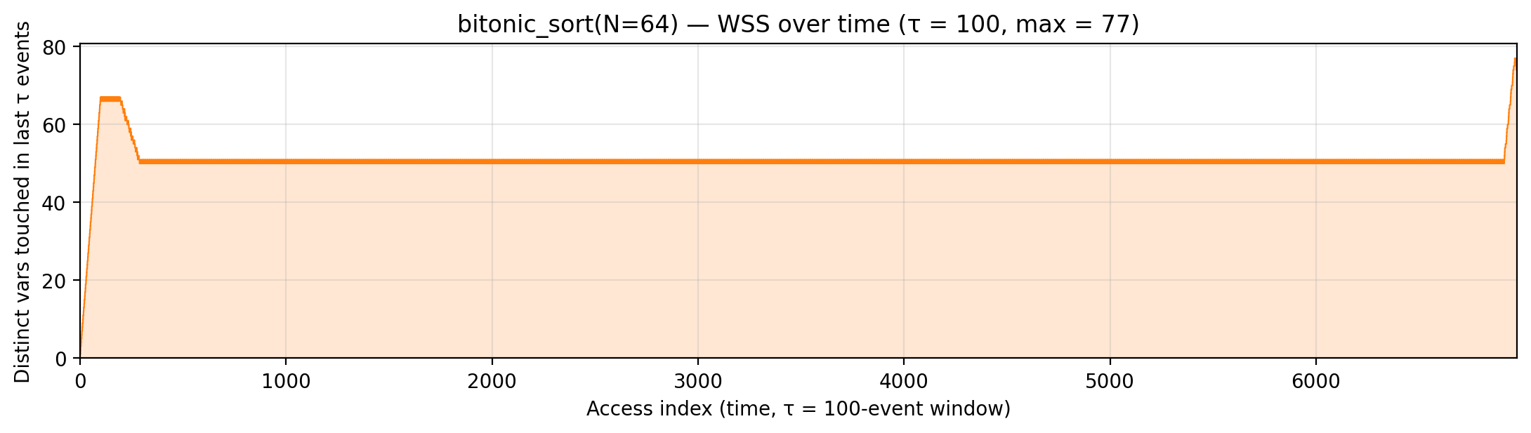
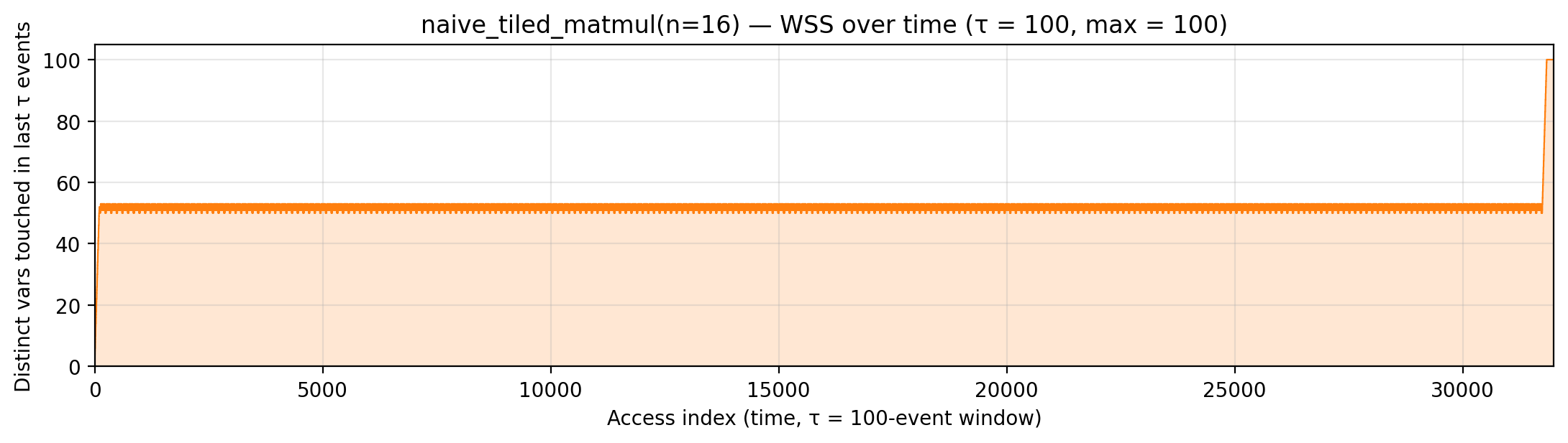
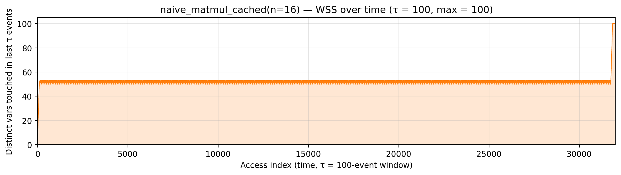
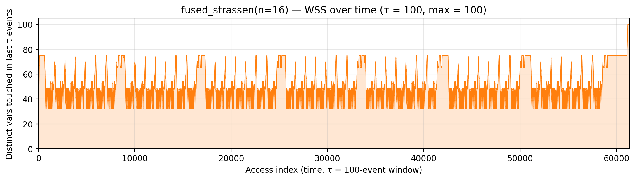
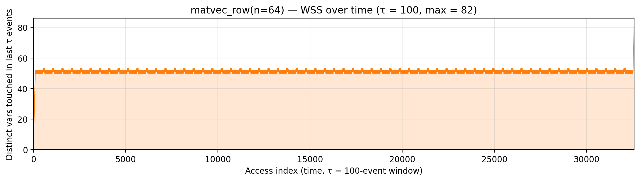
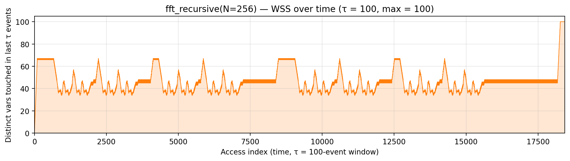
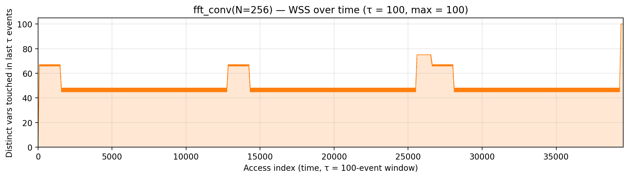
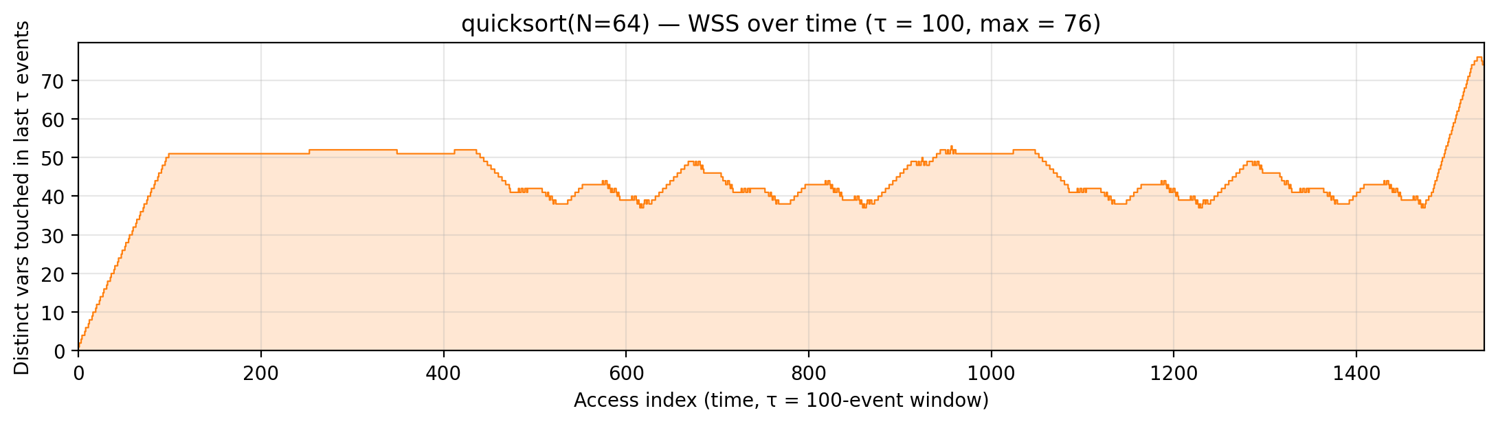
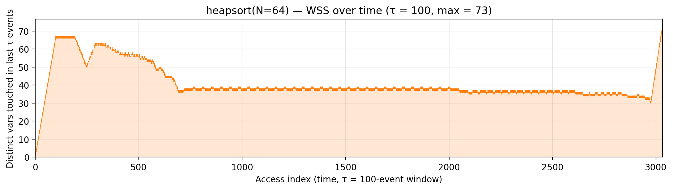
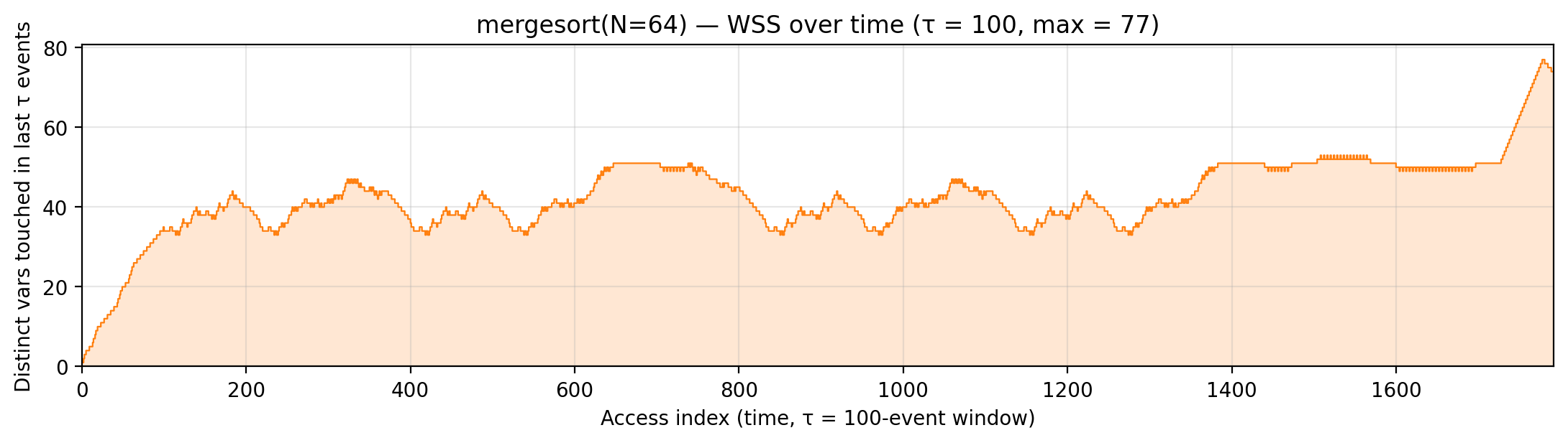
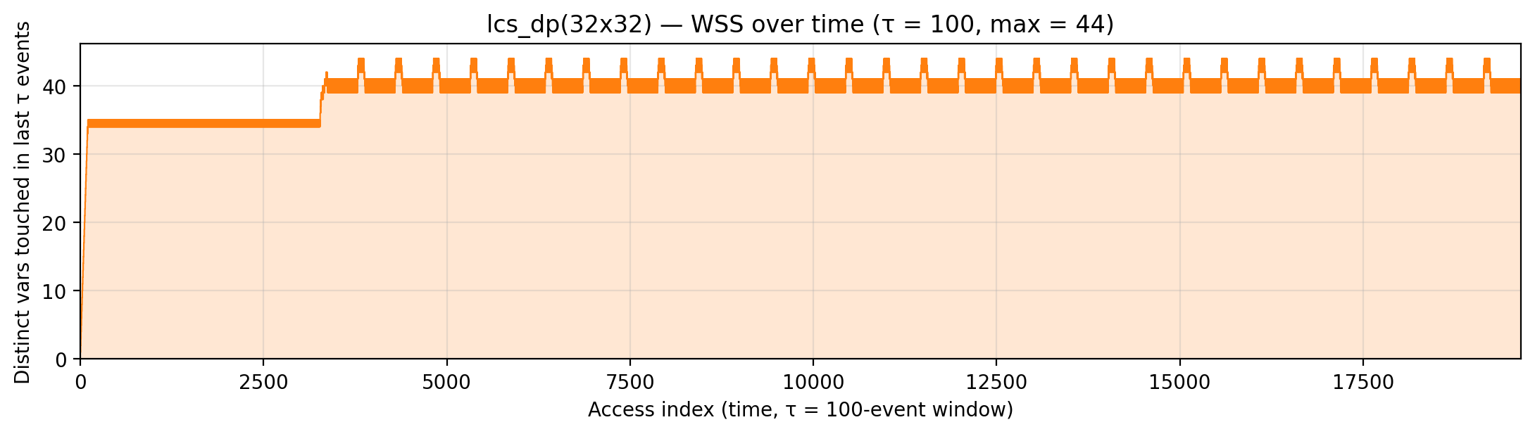
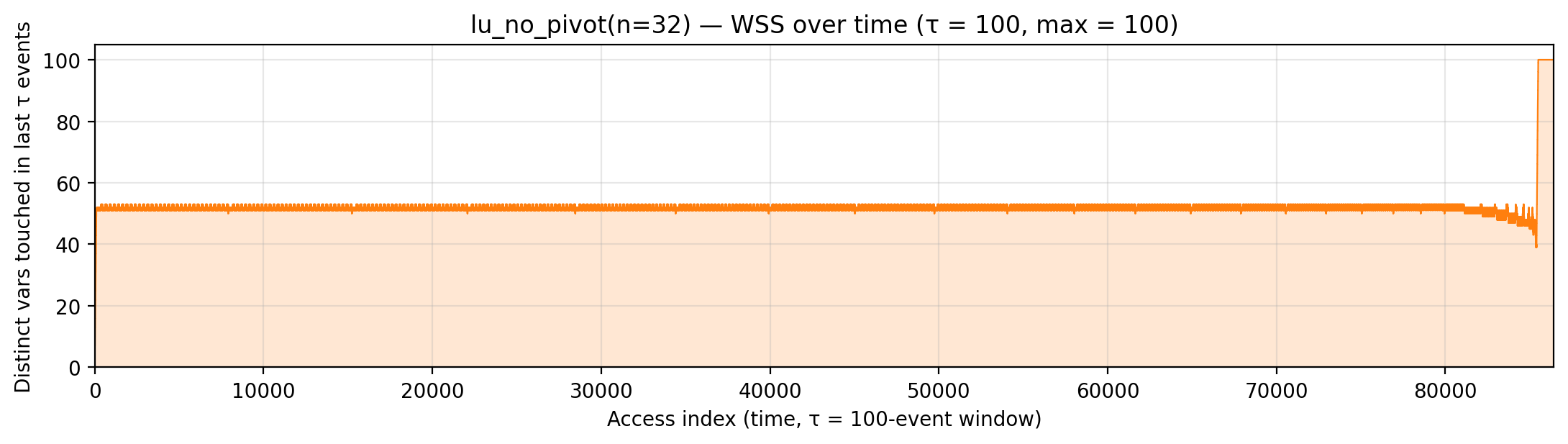
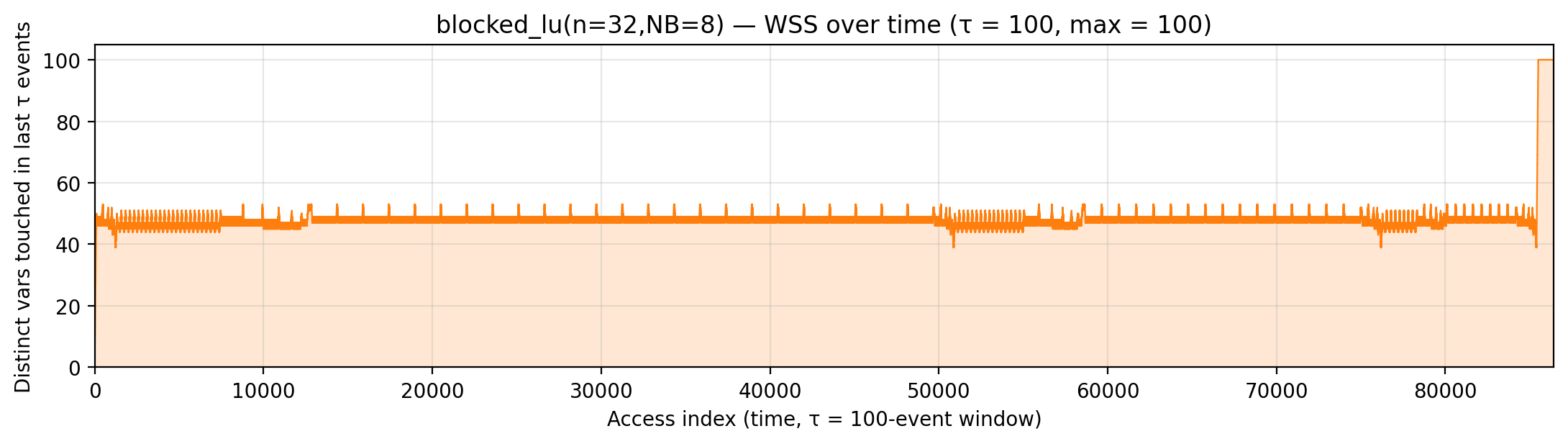
<slug>_wss.png |
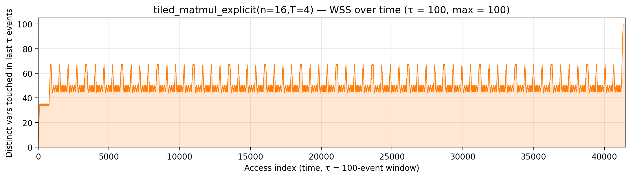
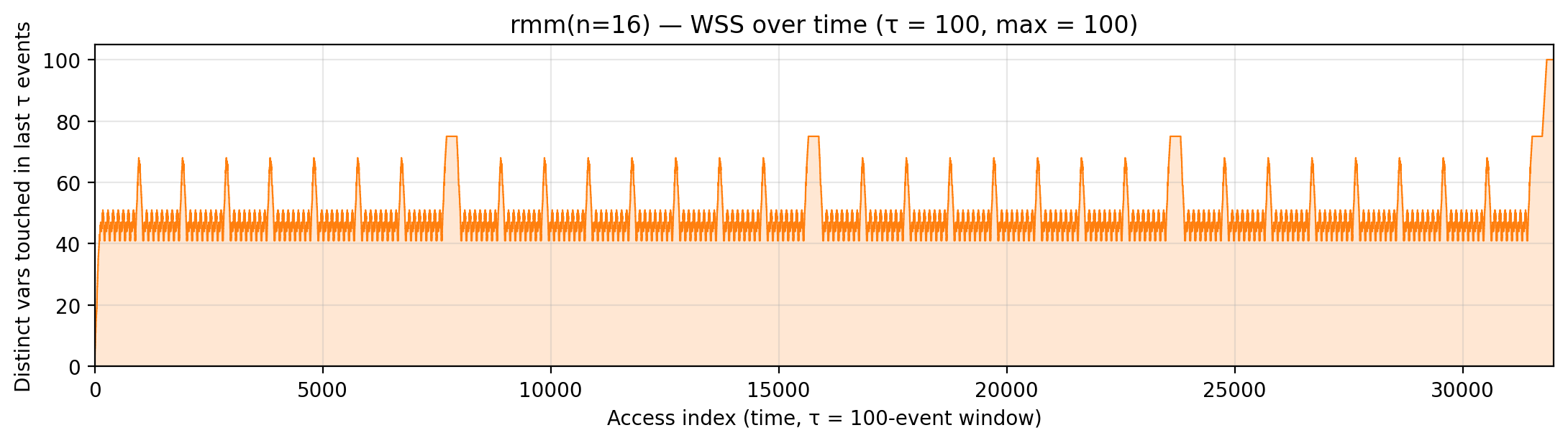
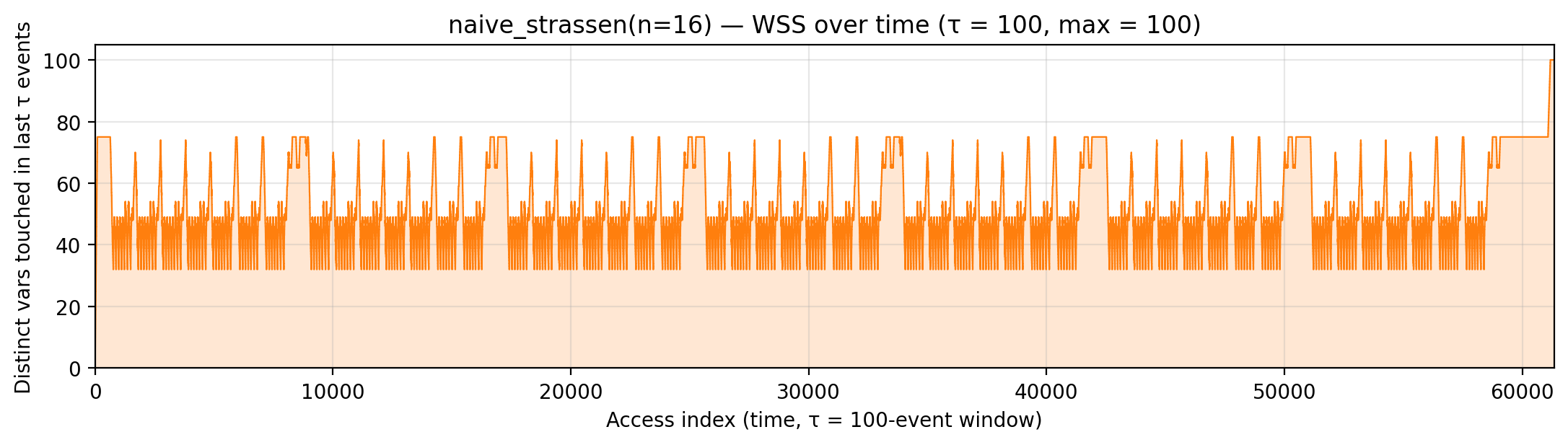
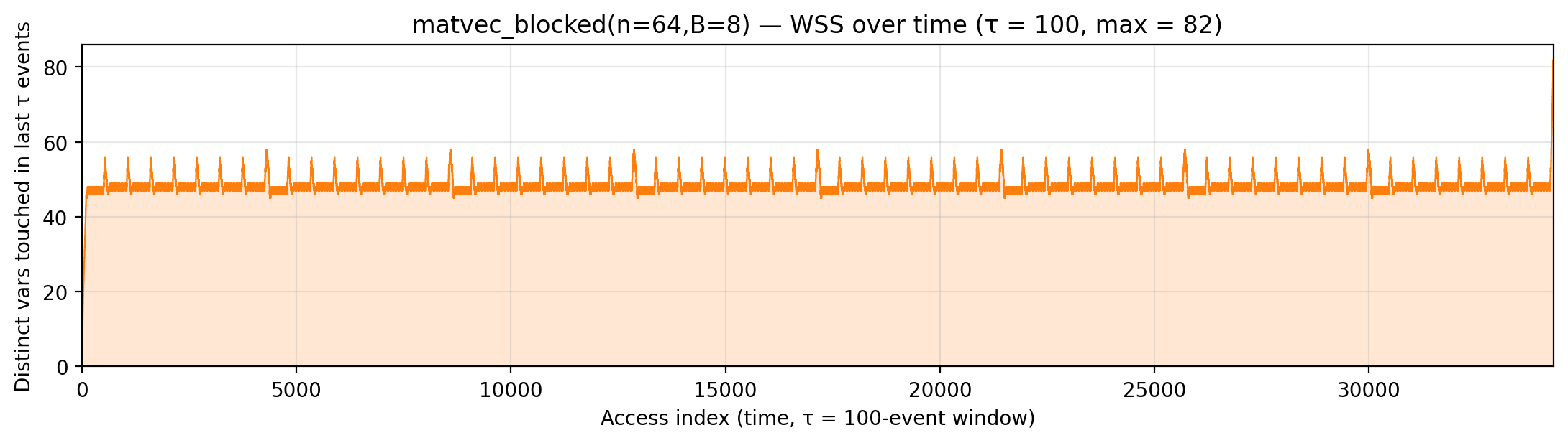
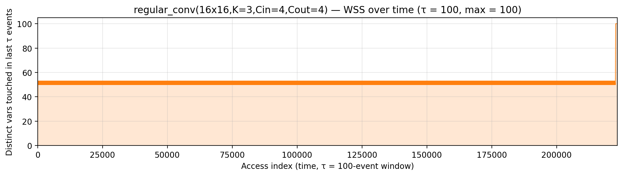
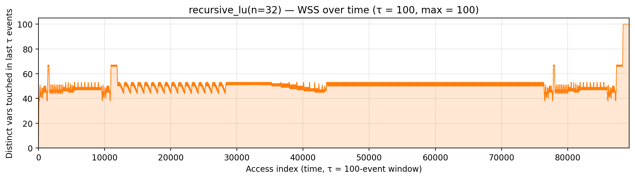
Sliding-τ working-set size (Denning 1968): number of distinct vars referenced inside a trailing τ-event window. τ is picked per-algorithm at the 90th-percentile reuse distance. | — |
All charts above are generated for every algorithm in roughly 3 seconds per algorithm; no chart is currently slow enough to skip (none “timed out” — the entire grid regenerates in ~2.7 minutes including the per-tick TU floor and OPT pass).
Notes
- MAC convention for the matmul family (naive/tiled/rmm/strassen
variants): accumulator read once per (i,j) outside the k-loop; 2 reads
(A, B) per k-iter. Matches
strassen_trace.py/efficient_strassen_trace.py—rmmandfused_strassenreproduce those scripts’ outputs exactly (95,222 and 140,526 at n=16, T=4). - Hot-slot allocation matters a lot for
matvec: putting accumulatoryand inputxat addresses 1..2n cuts manual cost roughly in half compared to placing them after A. - Manual can exceed
bytedmd_classicformergesort(8,416 vs 4,344),fft_recursive(103,290 vs 63,195),lcs_dp(85,929 vs 47,066), and slightly forquicksort(3,974 vs 3,661). When temporaries are many and live briefly, or the working set is one large bulk region at high addresses, fixed-placement pays the full⌈√addr⌉on every access while LRU heuristics amortize via recency. Fixed Manhattan is not always an upper envelope. - Manual can beat
bytedmd_liveforfft_iterative(25,528 vs 44,212),fft_conv(138,238 vs 148,320), andfused_strassen(140,526 vs 173,919). A tight in-place layout that parks everything in the hot region short-circuits what any recency heuristic can model on the abstract trace. - Manual can fall below
global_densityon 15 of 48 rows. Worst cases (gap as % ofglobal_density):blocked_lu40 %,naive_attn39 %,stencil_time_diamond34 %,lu_no_pivot/lu_partial_pivot30 %+,tiled_matmul28 %,fft_conv25 %,recursive_lu/tsqr14 %. In every one of these the manual schedule implements a fused / streaming / in-place variant that the abstract trace does not — same arithmetic DAG semantically, but vastly fewer materialized intermediates:naive_attn: trace materializes the fullN×NS and P matrices (≈ 8,000 vars at N=64); manual streams row-by-row through oneN-cellc_S_rowbuffer.- LU family (
lu_no_pivot,blocked_lu,lu_partial_pivot,recursive_lu): trace creates fresh vars for every Schur- complement update; manual updates the trailing matrix in place (A[i][j] = A[i][j] − L_ik·U_kj). fused_strassen: trace materializes M₁..M₇; manual ZAFS folds the sub-additions into the L1 tile loads, so the M_k vars never exist on any stack.tiled_matmul/tiled_matmul_explicit: trace frommatmul_tiledmaterializes per-iteration tile-copy vars; manual uses register-blocked outer products against virtual tiles.stencil_time_diamond: trace creates a fresh var for every(t, i, j)write; manual rolling buffer overwrites in place.fft_conv,regular_conv: manual fuses transform / channel accumulation into the same scratch slot.global_densityis a true lower bound on the optimal static allocator for the traced DAG — but the manual schedules in this list are not implementing the traced DAG, they are implementing algorithmically equivalent in-place / fused variants whose effective trace is much smaller. The LP/Pigeonhole argument is unaffected; it just doesn’t apply to the algorithmmanualis actually executing.
- Theoretical sandwich on
manual. Under the⌈√addr⌉cost model, any correct manual placement is bounded on both sides bybytedmd_live:0.3849 · bytedmd_live ≤ manual ≤ 4.0 · bytedmd_live. The lower bound is a Sleator–Tarjan-style competitive-caching proof lifted to the continuous √d model (gemini/tarjan-bytedmd-lower-bound.md); the upper bound is the companion constant-factor analysis for an optimal DMA-managed scratchpad (gemini/bytedmd-upper-bound.md). Every row in the summary table sits inside this sandwich — the tightest (stencil_time_diamond,naive_attn,fft_conv) at ~0.59×bytedmd_live, still +53 % above the 0.3849× floor. An approachable walkthrough of why hand-placed scratchpads are mathematically optimal on a 2D spatial grid is in gemini/illustrative-matmul-tiled.md. —
naive_matmul (code)
n=16. Algorithm. Triple-nested-loop computing $C = A \cdot B^{\mathsf T}$:
C[i][j] = Σ_k A[i][k] · B[j][k]. Both A and B are traversed row-major
(contiguous) in the inner k-loop — the symmetric, cache-friendly twin
of the standard AB variant.
Manual placement (truly naive). No scratchpad caching. The only
scratch slot is a multiply-intermediate tmp; the accumulator is
C[i][j] itself (read-modify-write per inner k). A and B stay on the
arg stack for every access.
tmp (addr 1) — multiply intermediate (only scratchpad)
C (addrs 2..n²+1) — output, accumulated in place
Manual 177,744 — worse than every heuristic including
bytedmd_classic (181,258) in the same ballpark. This row is meant
to show how much caching is worth: see naive_matmul_cached for the
with-scratchpad variant that drops 35 % off this baseline.
Working-set size over time (peak = 512).
Reuse distance per load — LRU vs Bélády OPT (max LRU = 512; max OPT = 512).
Miss-ratio curve — LRU vs Bélády OPT misses by cache capacity.
Per-tick TU LP floor — integrand of global_density: Σ_i ρ_{(i)} · √i over currently-live vars, ranked by density; the area equals global_density.
Per-tick splitting LP floor — integrand of local_density: Σ_i ρ_{(i)} · √i over the currently-active per-burst virtual intervals; the area equals the geometric portion of local_density.
Per-tick polymatroid LP floor — integrand of polymatroid_lb: Σ_v reads_v · ⌈√d_v⌉ / lifespan(v) over live vars, where d_v is each variable’s LP-implied static depth (gemini/polymatroid-relaxation.md). The area equals the geometric portion of polymatroid_lb.
Rolling spatial intensity — heartbeat plot of ops / Σ ⌈√d⌉ over a sliding window.
Cumulative compute vs fetch cost — slope = instantaneous spatial arithmetic intensity.
Gravity well — per-load fetch-cost ⌈√d⌉ scatter.
Spatial locality CDF — compute-fulfillment as a function of radius.
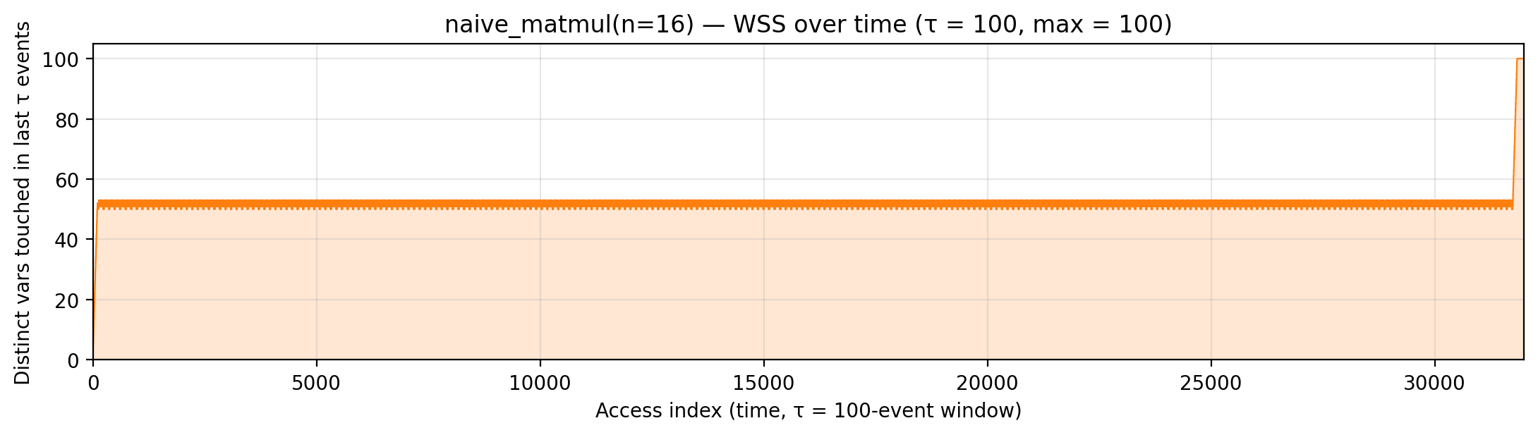
Working-set size over a τ = 100-event window (max = 100).
naive_2d_tiled_matmul (code)
n=16, T=4. Algorithm. Same triple-nested matmul as naive_matmul
— $C = A \cdot B^{\mathsf T}$ with $C[i][j] = \Sigma_k A[i][k] \cdot
B[j][k]$ — but with (i, j) iterated in tile-blocked order
$b_i \to b_j \to i_i \to j_j \to k$ instead of row-major. Each
$C[i][j]$ is still fully accumulated over all $k$ before moving on
and no scratchpad caching of A or B rows is introduced;
semantically identical to naive_matmul, only the visit order of
$(i, j)$ changes. This is pure output-only (“partitioned”) tiling.
Manual placement. Identical layout to naive_matmul:
tmp (addr 1) — multiply intermediate
C (addrs 2..n²+1) — output, accumulated in place
Because the multiset of accesses (which addresses, how many times) is
unchanged, the fixed-placement cost is identical: manual = 177,744
= naive_matmul’s. Reordering a loop can’t move addresses, so it can’t
change a ⌈√addr⌉-priced static schedule.
What tile-ordering alone buys. The recency-based heuristics do see the reordering:
| metric | naive_matmul | naive_2d_tiled | Δ |
|---|---|---|---|
manual |
177,744 | 177,744 | 0 |
global_density |
76,207 | 89,266 | +17 % |
local_density |
75,666 | 66,011 | −13 % |
polymatroid_lb |
— | — | both > 10 s budget |
bytedmd_opt |
111,388 | 95,571 | −14 % |
bytedmd_live |
109,473 | 95,890 | −12 % |
bytedmd_classic |
186,017 | 167,585 | −10 % |
Tile blocking reuses the same T rows of A across T values of $j_j$
(and the same T rows of B across T values of $i_i$) inside each
$(b_i, b_j)$ block, so LRU reuse distances for those rows collapse
from ≈ N² (naive’s full sweep) to ≈ N·T. global_density ticks up
because the time-integrated relaxation pays for the larger live-set
during these clustered bursts even when the load events themselves
are spaced out. Consequently, this row is useful as a clean baseline:
“what does tile-blocking the loop nest alone do?”, isolated from the
caching/scratchpad effects of naive_tiled_matmul (which actually
cuts arg traffic) and naive_matmul_cached (which hoists an A row
into a hot buffer).
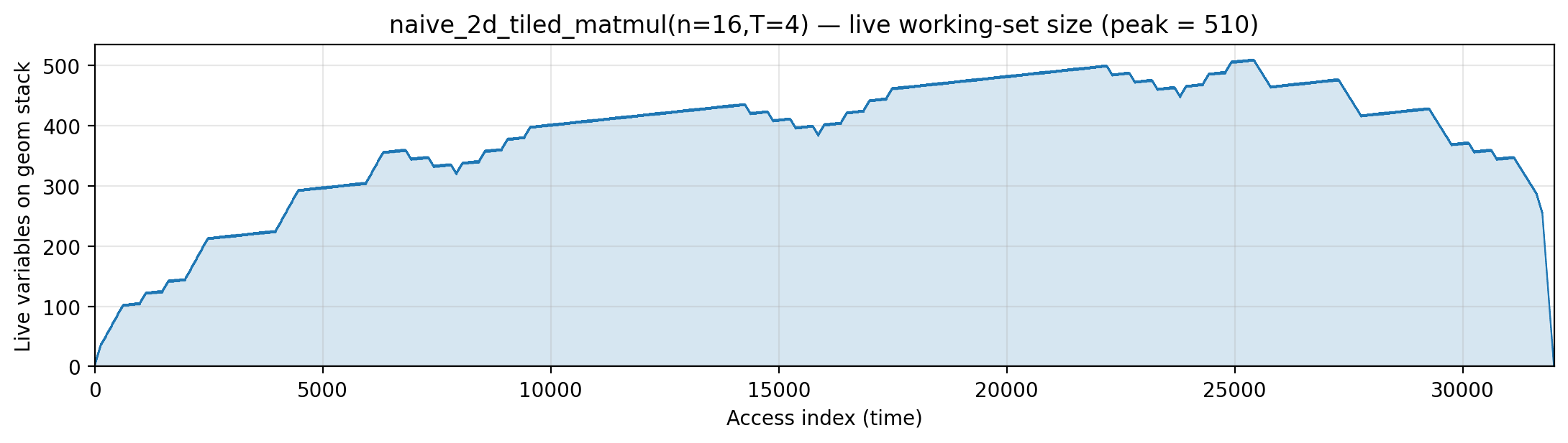
Working-set size over time (peak = 510).
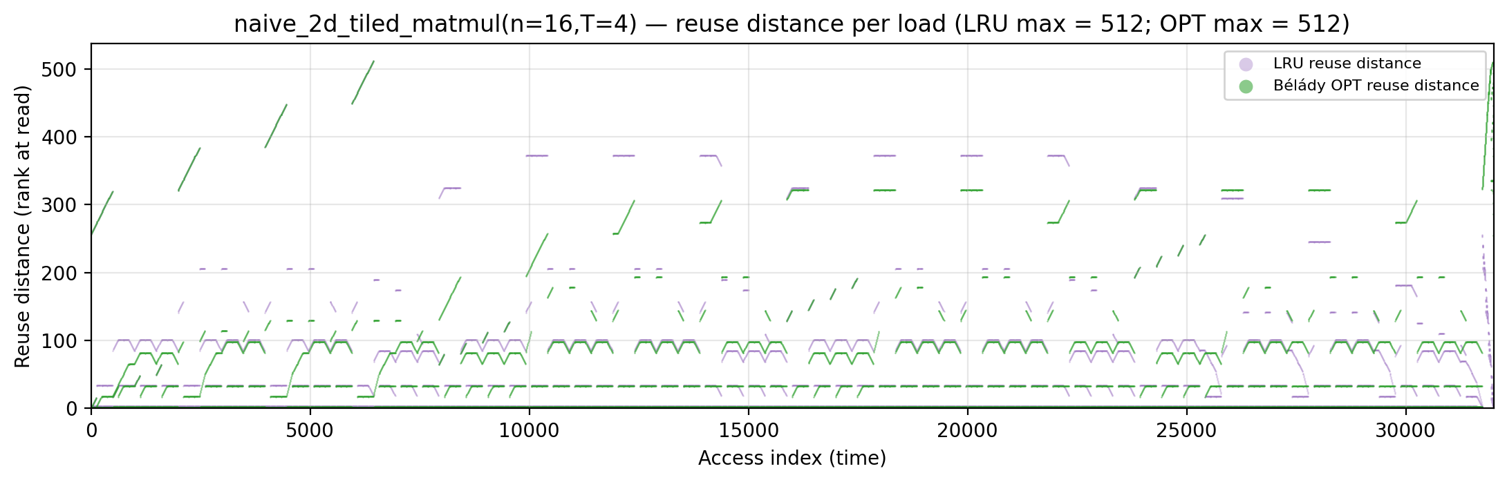
Reuse distance per load — LRU vs Bélády OPT (max LRU = 512; max OPT = 512).
Miss-ratio curve — LRU vs Bélády OPT misses by cache capacity.

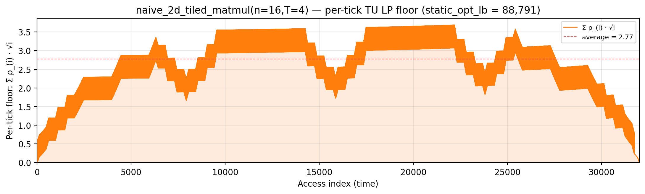
Per-tick TU LP floor — integrand of global_density: Σ_i ρ_{(i)} · √i over currently-live vars, ranked by density; the area equals global_density.
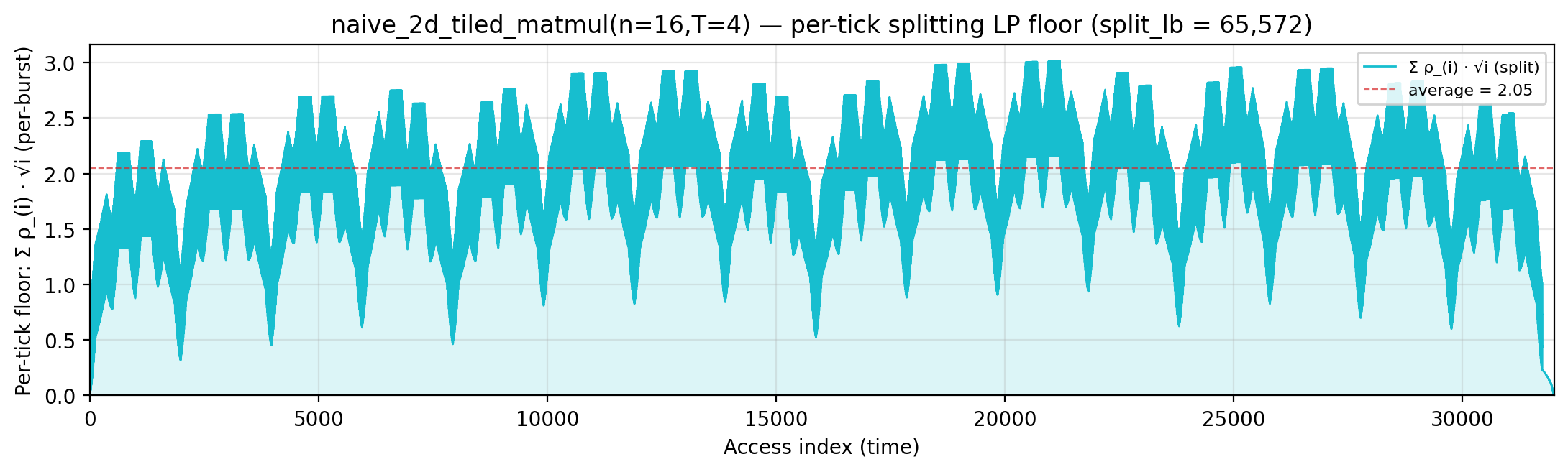
Per-tick splitting LP floor — integrand of local_density: Σ_i ρ_{(i)} · √i over the currently-active per-burst virtual intervals; the area equals the geometric portion of local_density.
Per-tick polymatroid LP floor — integrand of polymatroid_lb: Σ_v reads_v · ⌈√d_v⌉ / lifespan(v) over live vars, where d_v is each variable’s LP-implied static depth (gemini/polymatroid-relaxation.md). The area equals the geometric portion of polymatroid_lb.

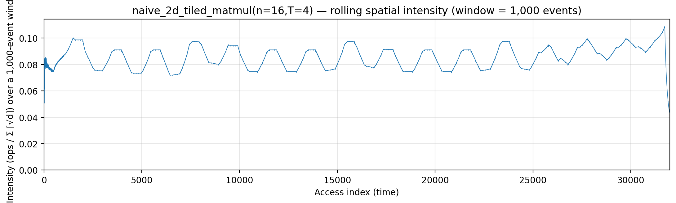
Rolling spatial intensity — heartbeat plot of ops / Σ ⌈√d⌉ over a sliding window.
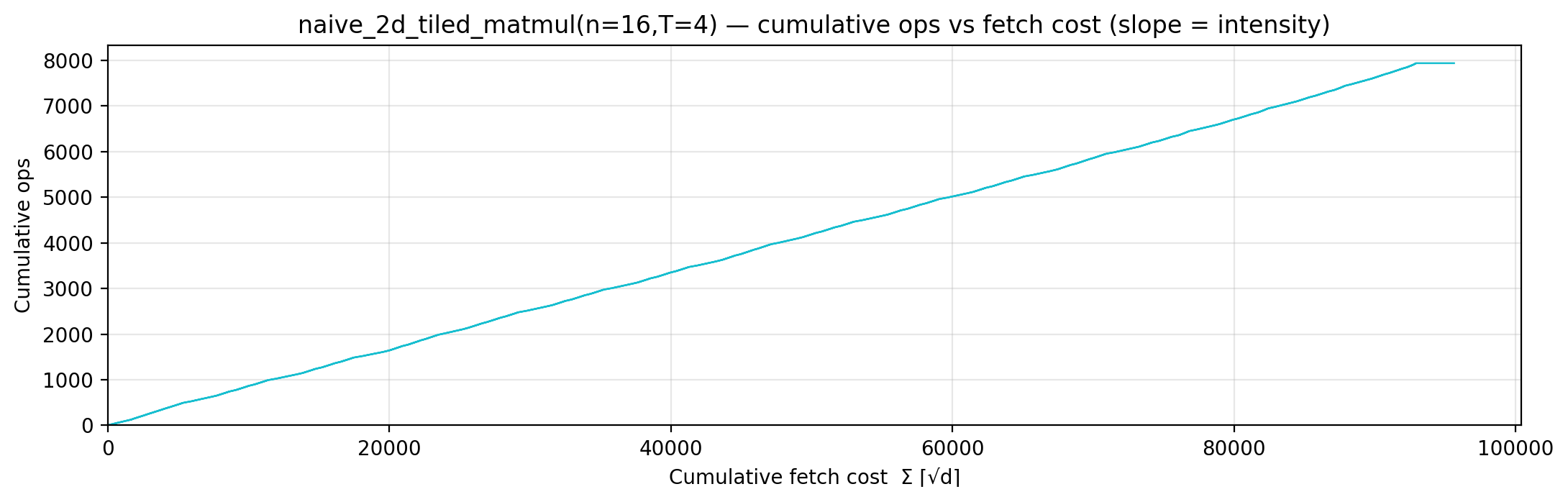
Cumulative compute vs fetch cost — slope = instantaneous spatial arithmetic intensity.
Gravity well — per-load fetch-cost ⌈√d⌉ scatter.

Spatial locality CDF — compute-fulfillment as a function of radius.
Working-set size over a τ = 100-event window (max = 100).

naive_tiled_matmul (code)
n=16, k=4. Algorithm. Same matmul as naive_matmul but
each block caches k rows of A and k rows of B (in the
A·B^T formulation, B’s “rows” are the transposed operand’s
columns — semantically one slab per side) and computes k² output
entries per block as full n-wide dot products against those
two scratch slabs.
Manual placement.
tmp (addr 1) — multiply intermediate
sA (addrs 2..k·n+1) — k rows of A (64 cells at k=4)
sB (addrs k·n+2..2k·n+1) — k rows of B
C (above sB) — output / accumulator in place
Choice of k. A sweep of k ∈ {1, 2, 4, 8, 16} for n=16:
| k | manual cost |
|---|---|
| 1 | 177,688 (≈ truly-naive) |
| 2 | 154,384 |
| 4 | 161,084 ← chosen |
| 8 | 191,202 |
| 16 | 245,693 |
Larger k amortizes arg reloads over more scratch reads but pushes
the scratch footprint deeper — at k=16 both matrices sit fully
in scratch and each sA/sB read pays sqrt(512). Smaller k is
near-no-op. k=4 doubles the block footprint over the minimum and
still gives a meaningful win: 4×4 = 16 output entries per block
with k·n = 64-cell scratch slabs.
Drops manual 177,744 → 161,084 (−9 %). Still above
naive_matmul_cached (114,838) because the A-row hoist there
keeps all of A[i][*] hot across every j for fixed i (stronger
reuse than a square tile), and well above tiled_matmul (67,758)
which adds register-level stationary-operand scheduling on top.
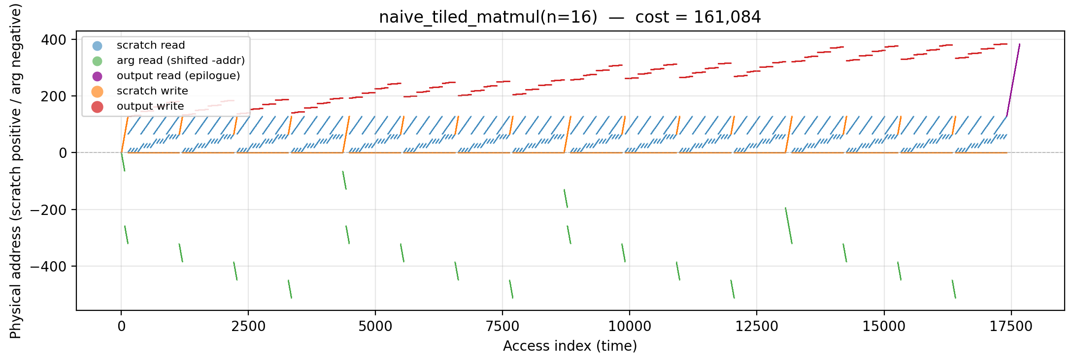
Working-set size over time (peak = 512).
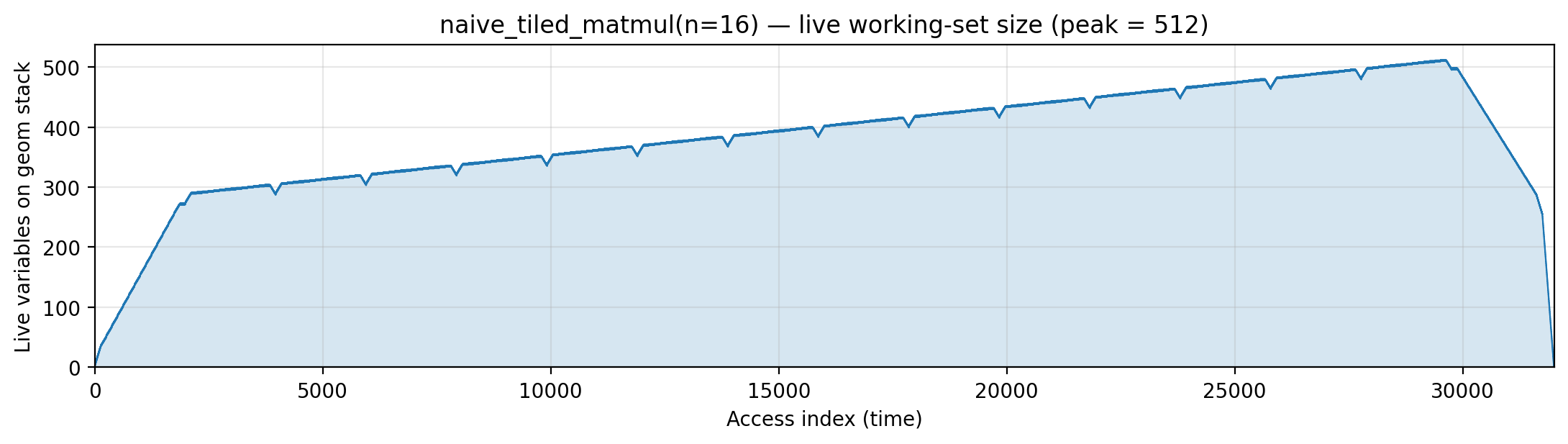
Reuse distance per load — LRU vs Bélády OPT (max LRU = 512; max OPT = 512).
Miss-ratio curve — LRU vs Bélády OPT misses by cache capacity.
Per-tick TU LP floor — integrand of global_density: Σ_i ρ_{(i)} · √i over currently-live vars, ranked by density; the area equals global_density.
Per-tick splitting LP floor — integrand of local_density: Σ_i ρ_{(i)} · √i over the currently-active per-burst virtual intervals; the area equals the geometric portion of local_density.
Per-tick polymatroid LP floor — integrand of polymatroid_lb: Σ_v reads_v · ⌈√d_v⌉ / lifespan(v) over live vars, where d_v is each variable’s LP-implied static depth (gemini/polymatroid-relaxation.md). The area equals the geometric portion of polymatroid_lb.
Rolling spatial intensity — heartbeat plot of ops / Σ ⌈√d⌉ over a sliding window.
Cumulative compute vs fetch cost — slope = instantaneous spatial arithmetic intensity.
Gravity well — per-load fetch-cost ⌈√d⌉ scatter.
Spatial locality CDF — compute-fulfillment as a function of radius.
Working-set size over a τ = 100-event window (max = 100).
naive_matmul_cached (code)
n=16. Algorithm. Same triple-nested-loop as naive_matmul.
Manual placement. A[i][*] is reused across all n values of j for
fixed outer i — preloading it once per i into c_A_row cuts n−1
redundant arg reads per A cell:
s (addr 1) — accumulator
c_A_row (addrs 2..n+1) — hot A[i][*] row buffer
C (addrs n+2..n+n²+1) — output
B[j][*] isn’t cached (would need reload for every i, wiping the win).
Drops manual 177,744 → 114,838 (−35 %) relative to the truly
naive variant. Still above bytedmd_live (111,098) because the
fully-tiled variant (tiled_matmul, which caches both tiles) is
what closes the gap further.
Working-set size over time (peak = 512).
Reuse distance per load — LRU vs Bélády OPT (max LRU = 512; max OPT = 512).
Miss-ratio curve — LRU vs Bélády OPT misses by cache capacity.
Per-tick TU LP floor — integrand of global_density: Σ_i ρ_{(i)} · √i over currently-live vars, ranked by density; the area equals global_density.
Per-tick splitting LP floor — integrand of local_density: Σ_i ρ_{(i)} · √i over the currently-active per-burst virtual intervals; the area equals the geometric portion of local_density.
Per-tick polymatroid LP floor — integrand of polymatroid_lb: Σ_v reads_v · ⌈√d_v⌉ / lifespan(v) over live vars, where d_v is each variable’s LP-implied static depth (gemini/polymatroid-relaxation.md). The area equals the geometric portion of polymatroid_lb.
Rolling spatial intensity — heartbeat plot of ops / Σ ⌈√d⌉ over a sliding window.
Cumulative compute vs fetch cost — slope = instantaneous spatial arithmetic intensity.
Gravity well — per-load fetch-cost ⌈√d⌉ scatter.
Spatial locality CDF — compute-fulfillment as a function of radius.
Working-set size over a τ = 100-event window (max = 100).
tiled_matmul (code)
n=16, T=4. Algorithm. One-level blocked matmul — iterate over
(bi, bj, bk) tiles of size T×T, compute each inner tile with the triple
loop. Same arithmetic as naive but in block-major order for locality.
Why does the manual score here beat
bytedmd_liveoutright? See the audit note in gemini/tiled-matmul-optimization.md — it’s not an accounting cheat; the manual schedule implements a fundamentally different register-blocked outer product (B-row stationary,blocks=2) that the trace-based heuristics score against the naive 2D-tiling Python code.
Manual placement. Register-blocked outer product with a B-row
stationary schedule (gemini/optimized-tiled-matmul.md)
plus two last-mile micro-optimizations
(gemini/optimize-tiling-to-death.md):
c_A (addr 1) — hottest scalar (4,096 touches);
tmp (addr 2) — multiply intermediate (3,840 touches);
c_B (addrs 3..T+2) — L1 vector holding the current row of B;
sC (addrs T+3..T+2+blocks·T²) — 2D accumulator for TWO vertical
C tiles simultaneously so each B-row fetch is amortized.
The two micro-wins: (a) frequency-first allocation — c_A
(4,096 touches) locks in at address 1 instead of tmp (3,840
touches), saving 256 cost units; (b) first-MAC bypass — on
the very first accumulator write (bk=0, kk=0) write the mul
result directly into sC instead of the redundant tmp → sC
round-trip, saving another 256. Together they drop manual
68,270 → 67,758, which the gemini note argues is the strict
AM-GM lower bound for this scratchpad geometry
(C₁·N³·√S + C₂·N³/√S ≥ 2N³√(C₁C₂), minimized at the 8×4
accumulator footprint realised here). Below both other heuristics
(bytedmd_live 78,708, bytedmd_classic 143,812).
Working-set size over time (peak = 500).
Reuse distance per load — LRU vs Bélády OPT (max LRU = 512; max OPT = 512).
Miss-ratio curve — LRU vs Bélády OPT misses by cache capacity.
Per-tick TU LP floor — integrand of global_density: Σ_i ρ_{(i)} · √i over currently-live vars, ranked by density; the area equals global_density.
Per-tick splitting LP floor — integrand of local_density: Σ_i ρ_{(i)} · √i over the currently-active per-burst virtual intervals; the area equals the geometric portion of local_density.
Per-tick polymatroid LP floor — integrand of polymatroid_lb: Σ_v reads_v · ⌈√d_v⌉ / lifespan(v) over live vars, where d_v is each variable’s LP-implied static depth (gemini/polymatroid-relaxation.md). The area equals the geometric portion of polymatroid_lb.
Rolling spatial intensity — heartbeat plot of ops / Σ ⌈√d⌉ over a sliding window.
Cumulative compute vs fetch cost — slope = instantaneous spatial arithmetic intensity.
Gravity well — per-load fetch-cost ⌈√d⌉ scatter.
Spatial locality CDF — compute-fulfillment as a function of radius.
Working-set size over a τ = 147-event window (max = 147).
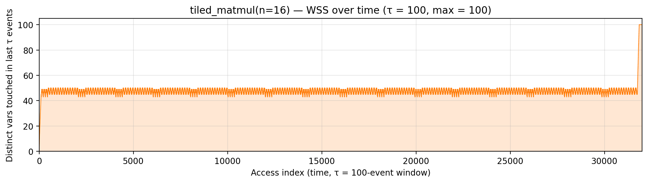
tiled_matmul_explicit (code)
n=16, T=4. Algorithm. Same arithmetic as tiled_matmul but with
explicit DMA materialization in the trace: before each tile’s MAC,
sA, sB, sC are populated by [... A[..] + 0.0 ...] comprehensions
that emit L2Load → L2Op("add") → L2Store(fresh_var) — creating
short-lived, high-density tile-local variables. At the end of each
(bi, bj) the final sC is flushed back to C via the same idiom.
Why this row exists. The original tiled_matmul reads directly
from A, B, C in the inner MAC; the trace never mentions a
scratchpad. The static-LP heuristics can only rank the actual traced
variables, so they’re stuck paying long-distance reads to A/B on
every inner iteration. The explicit version materializes the
scratchpad into the trace itself: the tile-local vars then sit near
Rank 1..3T² for any reasonable static layout.
Notice the LRU metrics go the other way: bytedmd_live climbs
74,560 → 97,486 and bytedmd_classic 143,280 → 203,220. LRU’s
dynamic recency bump was already building a scratchpad for free via
depth-1 promotion, so the extra DMA events just add cost without
offsetting benefit. This is the TPU / software-scratchpad vs
GPU / hardware-LRU framing: a static compiler benefits from
explicit DMA materialization, while a dynamic LRU cache does not.
Manual uses the same physical schedule as this explicit version, so
it has the same cost (67,758) — both “explicit” and “manual” land on
the TPU bound.
Working-set size over time (peak = 609).
Reuse distance per load — LRU vs Bélády OPT (max LRU = 576; max OPT = 512).
Miss-ratio curve — LRU vs Bélády OPT misses by cache capacity.
Per-tick TU LP floor — integrand of global_density: Σ_i ρ_{(i)} · √i over currently-live vars, ranked by density; the area equals global_density.
Per-tick splitting LP floor — integrand of local_density: Σ_i ρ_{(i)} · √i over the currently-active per-burst virtual intervals; the area equals the geometric portion of local_density.
Rolling spatial intensity — heartbeat plot of ops / Σ ⌈√d⌉ over a sliding window.
Cumulative compute vs fetch cost — slope = instantaneous spatial arithmetic intensity.
Gravity well — per-load fetch-cost ⌈√d⌉ scatter.
Spatial locality CDF — compute-fulfillment as a function of radius.
Working-set size over a τ = 144-event window (max = 144).
rmm (code)
n=16, T=4. Algorithm. Cache-oblivious recursive matmul: split each
of A, B, C into 4 quadrants and make 8 recursive calls (2×2×2 = 8
sub-products in Hamiltonian order), descending until sz = T where the
base-case tile kernel runs.
Manual placement. Same scratchpad+bulk layout as tiled. The recursion naturally generates a Hamiltonian walk over C-tiles; only the immediately-prior C tile is considered “loaded” (matches strassen_trace’s cache semantic), so 7 of 8 consecutive base calls reload C while 1 skips the pre-fetch.
Working-set size over time (peak = 554).
Reuse distance per load — LRU vs Bélády OPT (max LRU = 522; max OPT = 512).
Miss-ratio curve — LRU vs Bélády OPT misses by cache capacity.
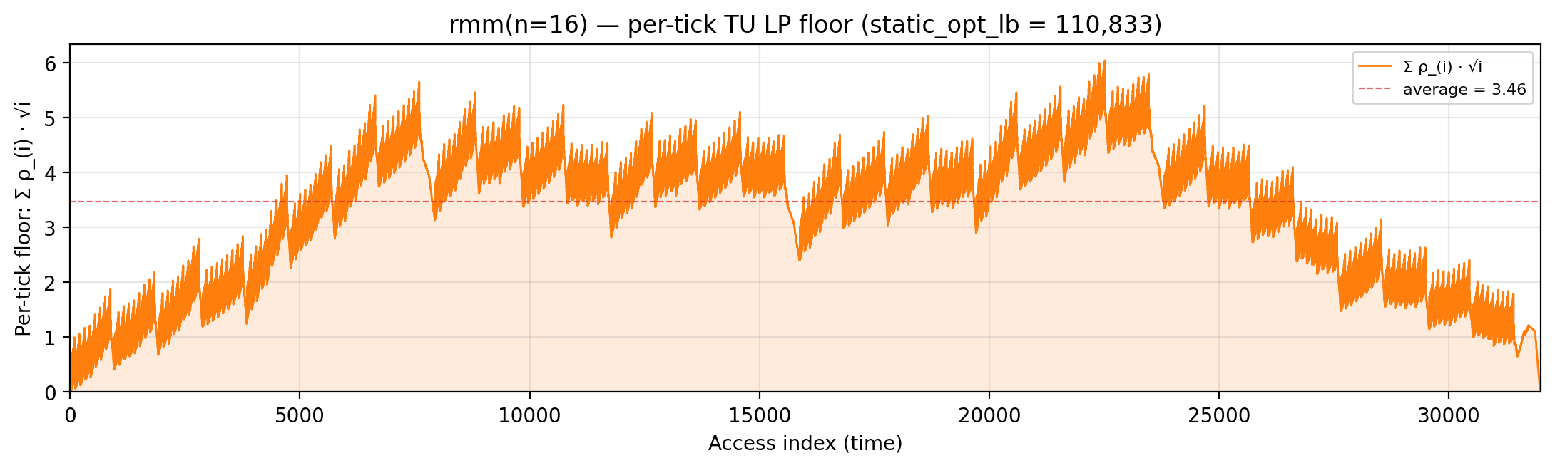
Per-tick TU LP floor — integrand of global_density: Σ_i ρ_{(i)} · √i over currently-live vars, ranked by density; the area equals global_density.
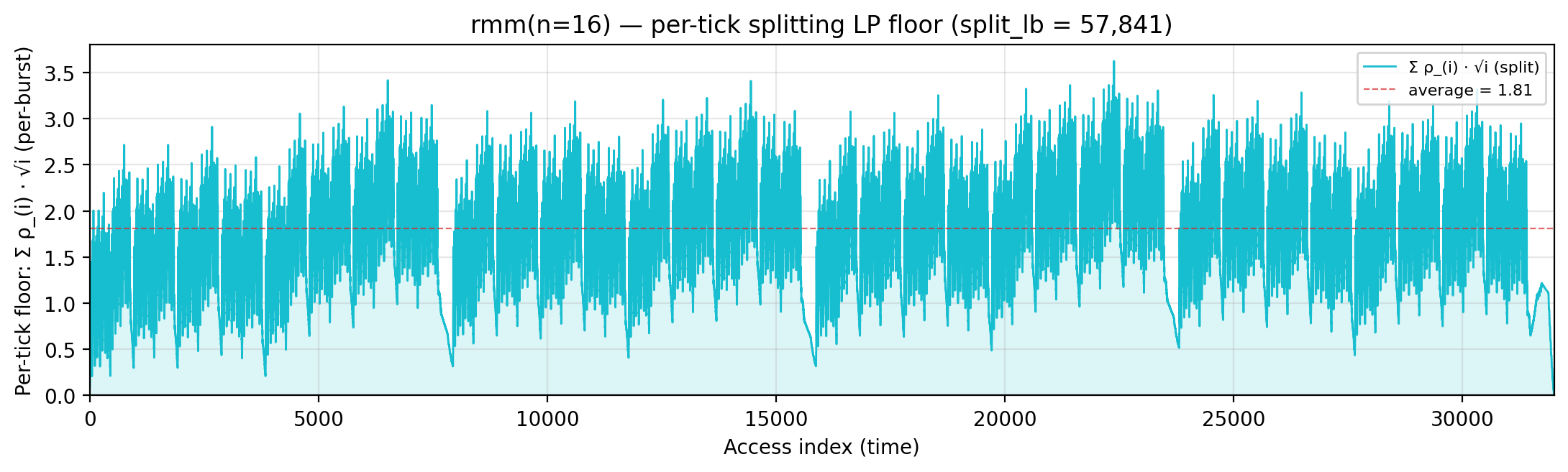
Per-tick splitting LP floor — integrand of local_density: Σ_i ρ_{(i)} · √i over the currently-active per-burst virtual intervals; the area equals the geometric portion of local_density.
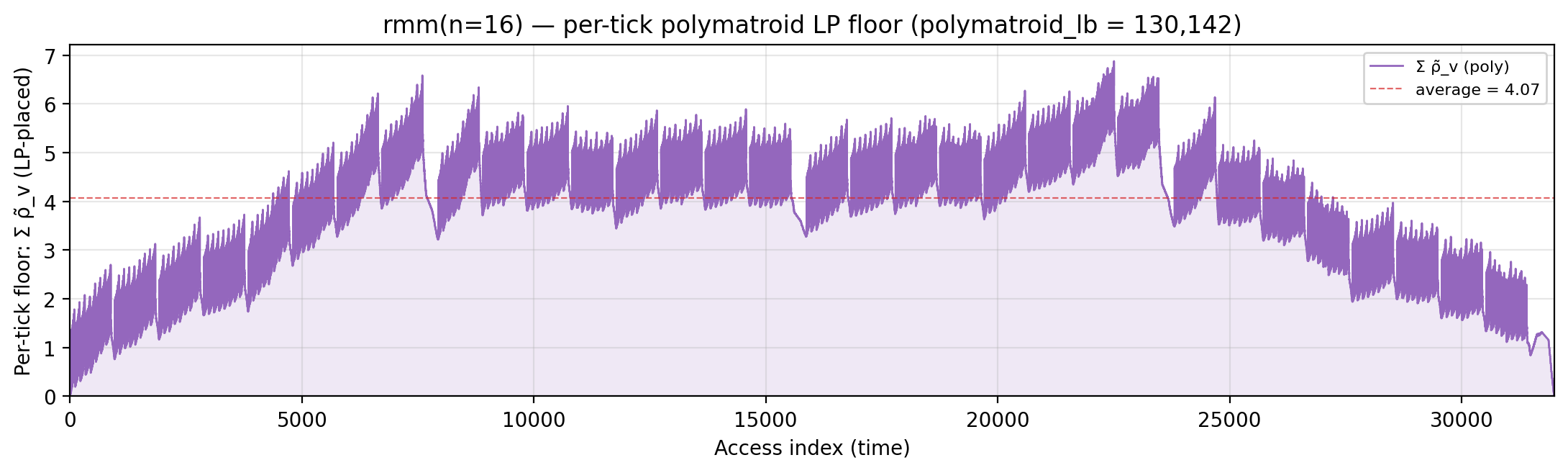
Per-tick polymatroid LP floor — integrand of polymatroid_lb: Σ_v reads_v · ⌈√d_v⌉ / lifespan(v) over live vars, where d_v is each variable’s LP-implied static depth (gemini/polymatroid-relaxation.md). The area equals the geometric portion of polymatroid_lb.
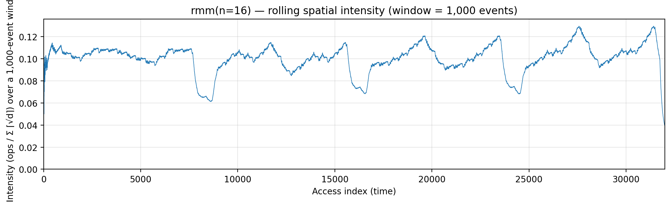
Rolling spatial intensity — heartbeat plot of ops / Σ ⌈√d⌉ over a sliding window.
Cumulative compute vs fetch cost — slope = instantaneous spatial arithmetic intensity.
Gravity well — per-load fetch-cost ⌈√d⌉ scatter.
Spatial locality CDF — compute-fulfillment as a function of radius.
Working-set size over a τ = 125-event window (max = 125).
naive_strassen (code)
n=16, T=4. Algorithm. Standard recursive Strassen: at each level
split A and B into 2×2 quadrants and compute 7 matrix products
$M_1 \ldots M_7$ (plus 10 matrix adds/subs), then assemble the 4 C
quadrants from linear combinations of the M matrices. Bottoms out at
T×T scratchpad tile kernels.
Manual placement. Scratchpads sA, sB, sC at the lowest addresses;
A, B, C bulk at addrs 3T²+1 onwards. Each recursion level uses
push/pop to allocate 7 temporary M matrices plus 2 sum buffers SA,
SB just above the current allocator pointer — so the pointer climbs
to ~9·h² extra slots per level before unwinding. Those M matrices are
where the cost goes: every read of M[i] during the assembly phase pays
full ⌈√addr⌉ on the stack-high region. Manual cost 282,382 is 2.01×
higher than fused_strassen (140,526) — the entire ZAFS win is the
avoidance of these materialized intermediates.
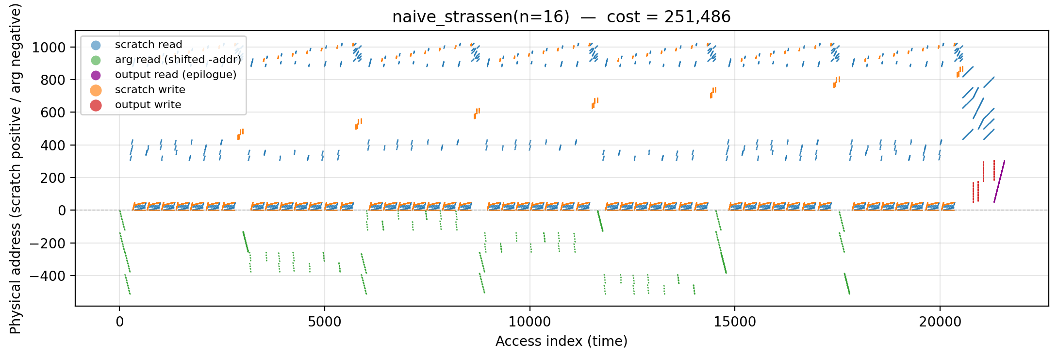
Working-set size over time (peak = 937).
Reuse distance per load — LRU vs Bélády OPT (max LRU = 768; max OPT = 596).
Miss-ratio curve — LRU vs Bélády OPT misses by cache capacity.
Per-tick TU LP floor — integrand of global_density: Σ_i ρ_{(i)} · √i over currently-live vars, ranked by density; the area equals global_density.
Per-tick splitting LP floor — integrand of local_density: Σ_i ρ_{(i)} · √i over the currently-active per-burst virtual intervals; the area equals the geometric portion of local_density.
Rolling spatial intensity — heartbeat plot of ops / Σ ⌈√d⌉ over a sliding window.
Cumulative compute vs fetch cost — slope = instantaneous spatial arithmetic intensity.
Gravity well — per-load fetch-cost ⌈√d⌉ scatter.
Spatial locality CDF — compute-fulfillment as a function of radius.
Working-set size over a τ = 158-event window (max = 158).
fused_strassen (code)
n=16, T=4. Algorithm. Zero-Allocation Fused Strassen (ZAFS):
single-level outer Strassen (7 matrix multiplies instead of 8) where the
sub-additions (A₁₁+A₂₂, etc.) are evaluated on-the-fly while loading
the L1 tile — the intermediate M matrices are never materialized. Each of
the 7 recipes is distributed directly into the target C quadrants with
sign. Inner MAC prices the multiply’s intermediate and per-k accumulator
read to close the earlier undercharge
(gemini/strassen-cheating-macc.md).
Manual placement. Only 3 L1 tile slots (fast_A, fast_B, fast_C at
addrs 1..3T²) plus A, B, C in main memory. No allocation of the 7 M
matrices — the ZAFS win shows up entirely here in manual (140,526 vs
353,901 for the naïve trace-based upper envelope).
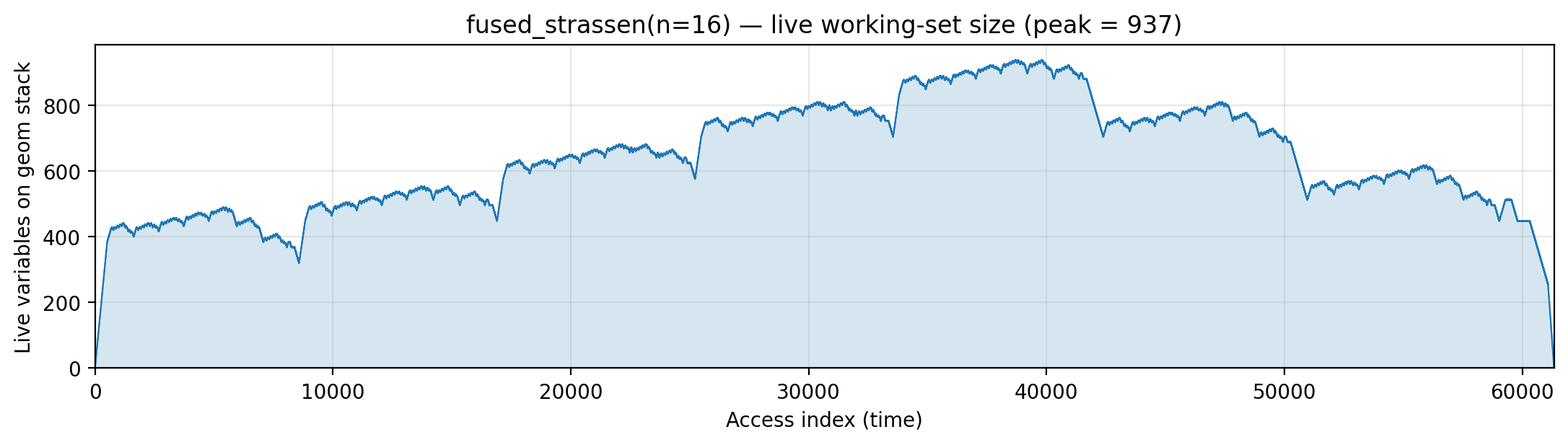
Working-set size over time (peak = 937).
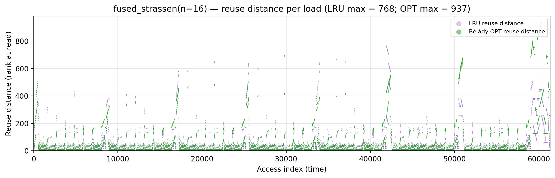
Reuse distance per load — LRU vs Bélády OPT (max LRU = 768; max OPT = 596).
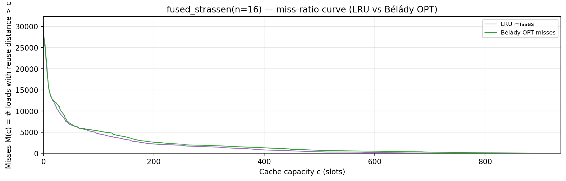
Miss-ratio curve — LRU vs Bélády OPT misses by cache capacity.
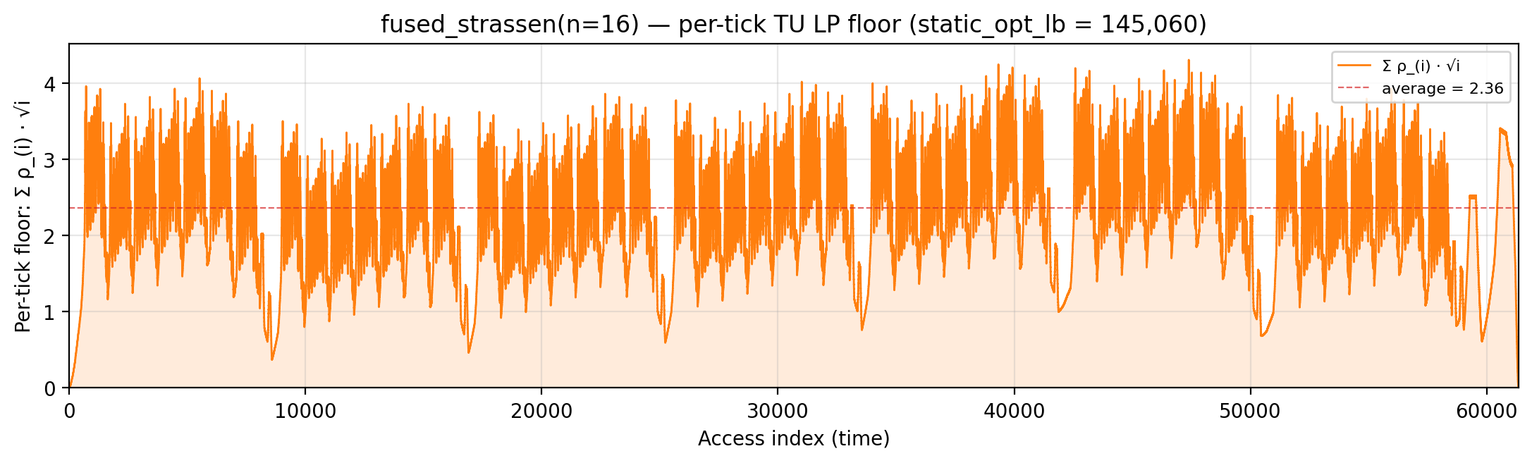
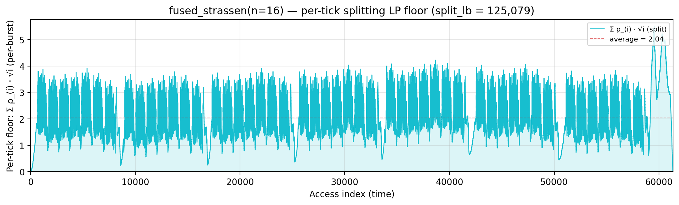
Per-tick TU LP floor — integrand of global_density: Σ_i ρ_{(i)} · √i over currently-live vars, ranked by density; the area equals global_density.
Per-tick splitting LP floor — integrand of local_density: Σ_i ρ_{(i)} · √i over the currently-active per-burst virtual intervals; the area equals the geometric portion of local_density.
Rolling spatial intensity — heartbeat plot of ops / Σ ⌈√d⌉ over a sliding window.
Cumulative compute vs fetch cost — slope = instantaneous spatial arithmetic intensity.
Gravity well — per-load fetch-cost ⌈√d⌉ scatter.
Spatial locality CDF — compute-fulfillment as a function of radius.
Working-set size over a τ = 158-event window (max = 158).
naive_attn (code)
N=64, d=2. Algorithm. Standard attention: compute full N×N
score matrix S = Q·Kᵀ/√d, row-wise softmax into P, then O = P·V.
The whole N×N matrix is materialized in memory.
Manual placement. Hot scalars s_acc, tmp, row_max, row_sum, inv_sum
at addrs 1..5; bulk Q, K, V (N·d each); the N² score/probability matrix
S (reused as P in-place); output O. The bulk S matrix dominates the
cost — every access pays ⌈√(addr ≈ N²)⌉.
Working-set size over time (peak = 4,164).
Reuse distance per load — LRU vs Bélády OPT (max LRU = 4,163; max OPT = 384).
Miss-ratio curve — LRU vs Bélády OPT misses by cache capacity.
Per-tick TU LP floor — integrand of global_density: Σ_i ρ_{(i)} · √i over currently-live vars, ranked by density; the area equals global_density.
Per-tick splitting LP floor — integrand of local_density: Σ_i ρ_{(i)} · √i over the currently-active per-burst virtual intervals; the area equals the geometric portion of local_density.
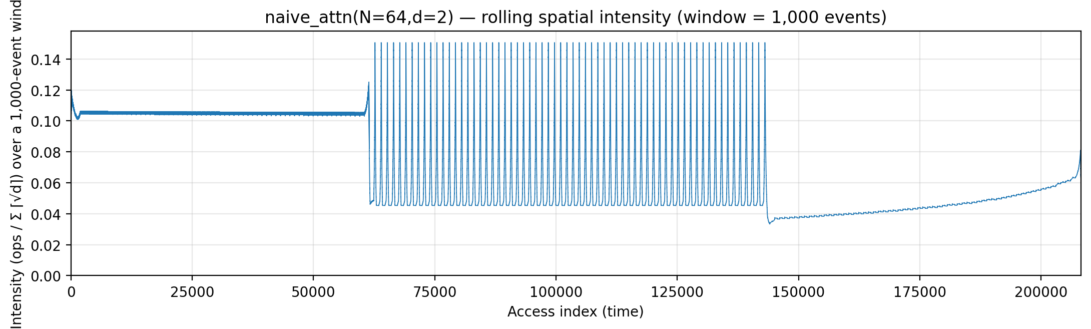
Rolling spatial intensity — heartbeat plot of ops / Σ ⌈√d⌉ over a sliding window.
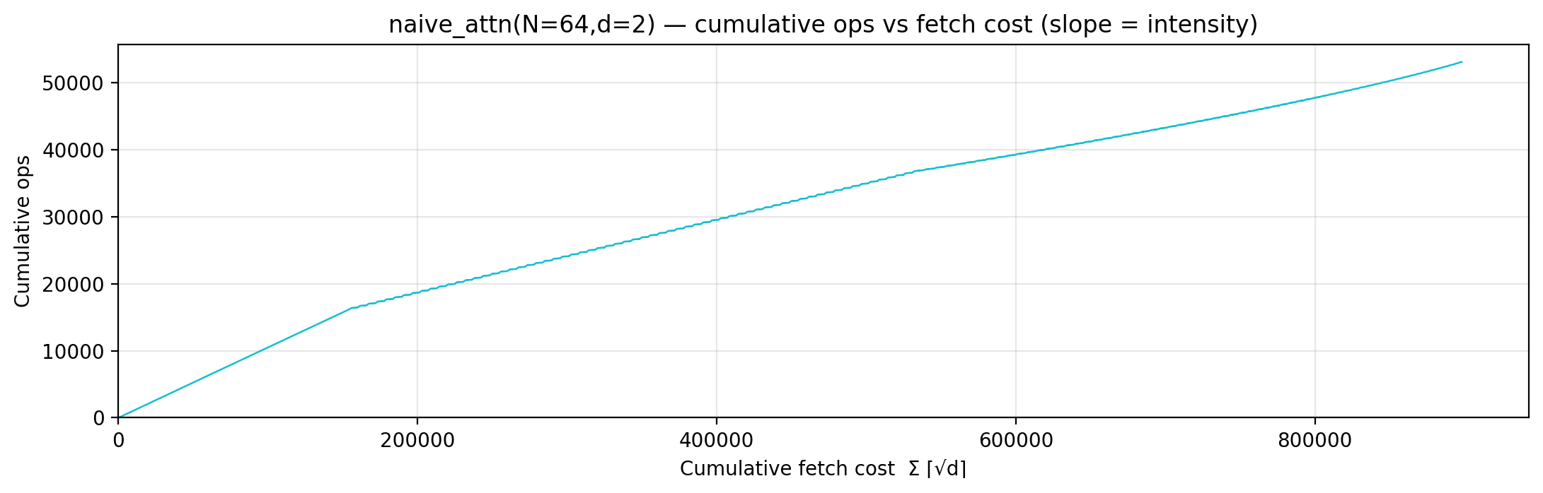
Cumulative compute vs fetch cost — slope = instantaneous spatial arithmetic intensity.
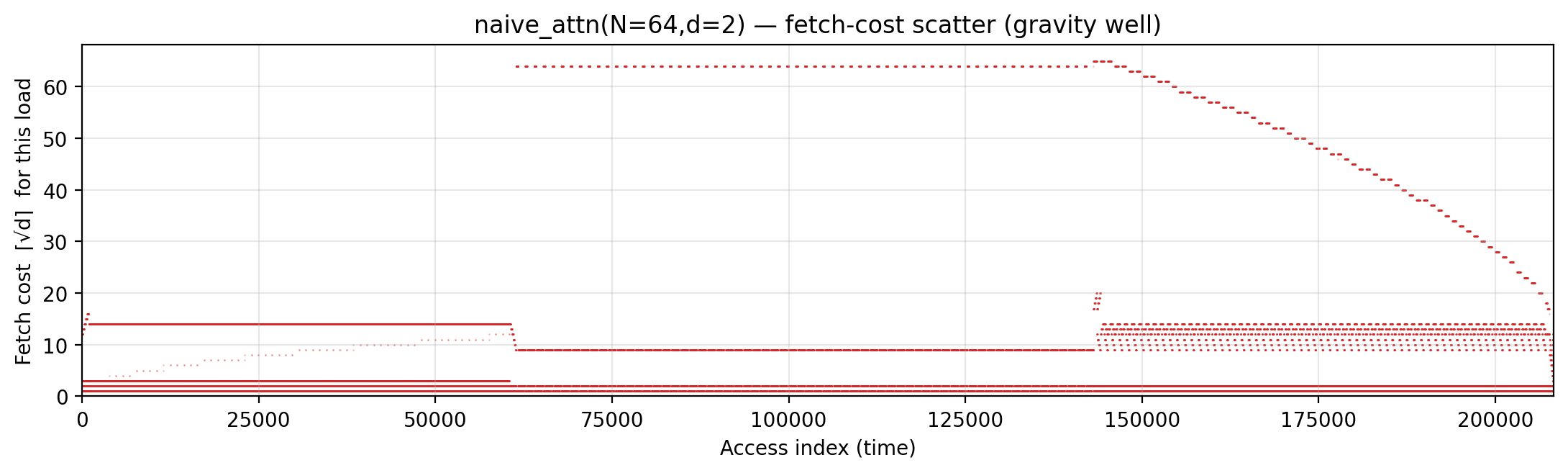
Gravity well — per-load fetch-cost ⌈√d⌉ scatter.
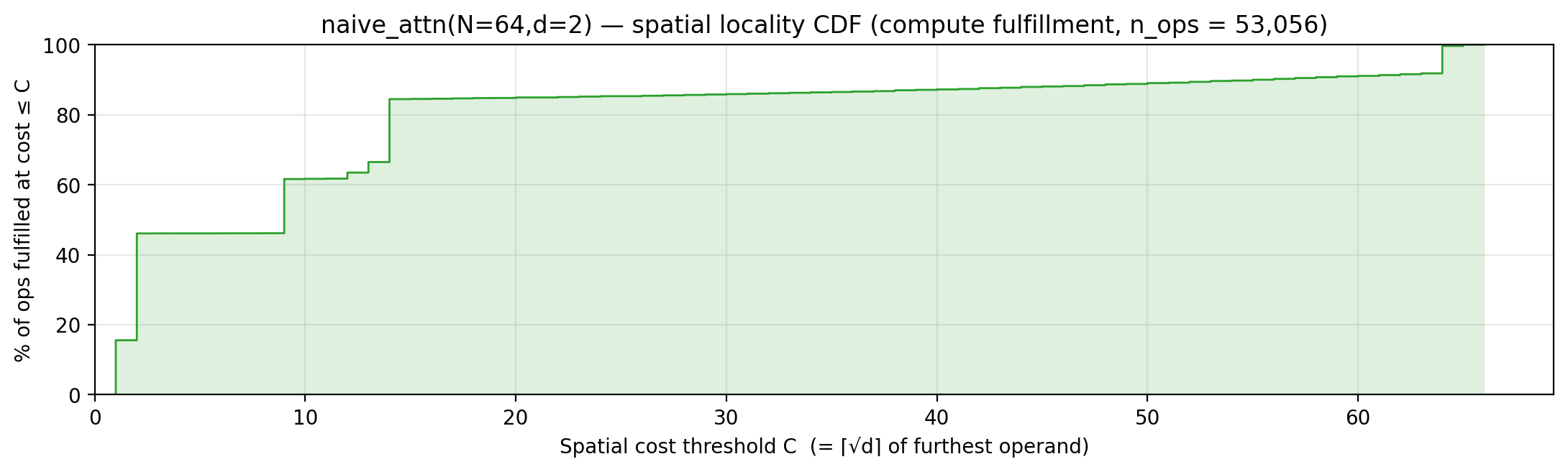
Spatial locality CDF — compute-fulfillment as a function of radius.
Working-set size over a τ = 100-event window (max = 100).
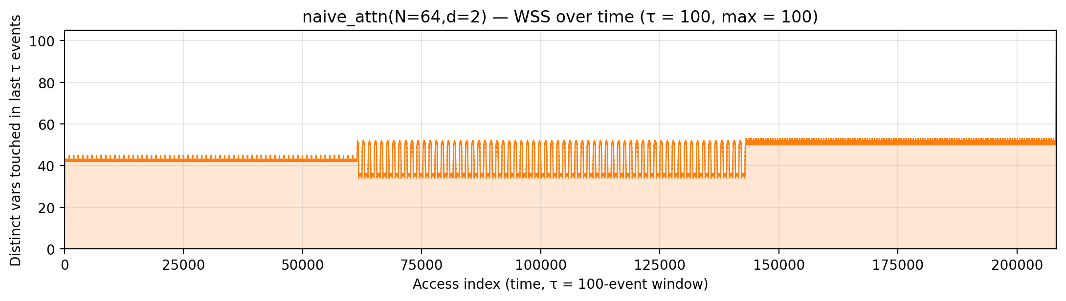
flash_attn (code)
N=64, d=2, Bk=8. Algorithm. Flash attention with online softmax
over K/V blocks of size Bk: for each query row, stream blocks of K and
V, compute block scores, update running (m, l) softmax stats, and
accumulate block contribution into o_acc. Never materializes the N×N
score matrix.
Manual placement. Bk-sized scratch blocks s_block, p_block and a
d-sized o_acc at low addrs; running m_i, l_i registers; merge
scalars m_block, l_block, m_new, α, β, inv_l, tmp also hot. At this
narrow head-dim (d=2), the manual naive schedule (532,805) beats the
manual flash schedule (610,154) by 15 %: the full N² S matrix is
small enough (4,096 cells) that it still sits within the cheap
sqrt(addr) region, so flash’s avoided-materialization win cannot
pay for its extra softmax-merge bookkeeping. The heuristics see the
flash win clearly — bytedmd_live 476k vs 898k — so flash would
win with a better hand-placement; the current manual is the outlier,
not the algorithm
(gemini/flash-attention-no-benefit.md,
gemini/naive-attention-surprise.md).
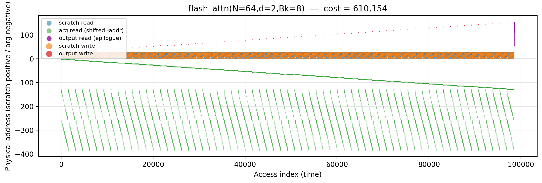
Working-set size over time (peak = 398).

Reuse distance per load — LRU vs Bélády OPT (max LRU = 384; max OPT = 384).

Miss-ratio curve — LRU vs Bélády OPT misses by cache capacity.
Per-tick TU LP floor — integrand of global_density: Σ_i ρ_{(i)} · √i over currently-live vars, ranked by density; the area equals global_density.
Per-tick splitting LP floor — integrand of local_density: Σ_i ρ_{(i)} · √i over the currently-active per-burst virtual intervals; the area equals the geometric portion of local_density.
Rolling spatial intensity — heartbeat plot of ops / Σ ⌈√d⌉ over a sliding window.
Cumulative compute vs fetch cost — slope = instantaneous spatial arithmetic intensity.
Gravity well — per-load fetch-cost ⌈√d⌉ scatter.
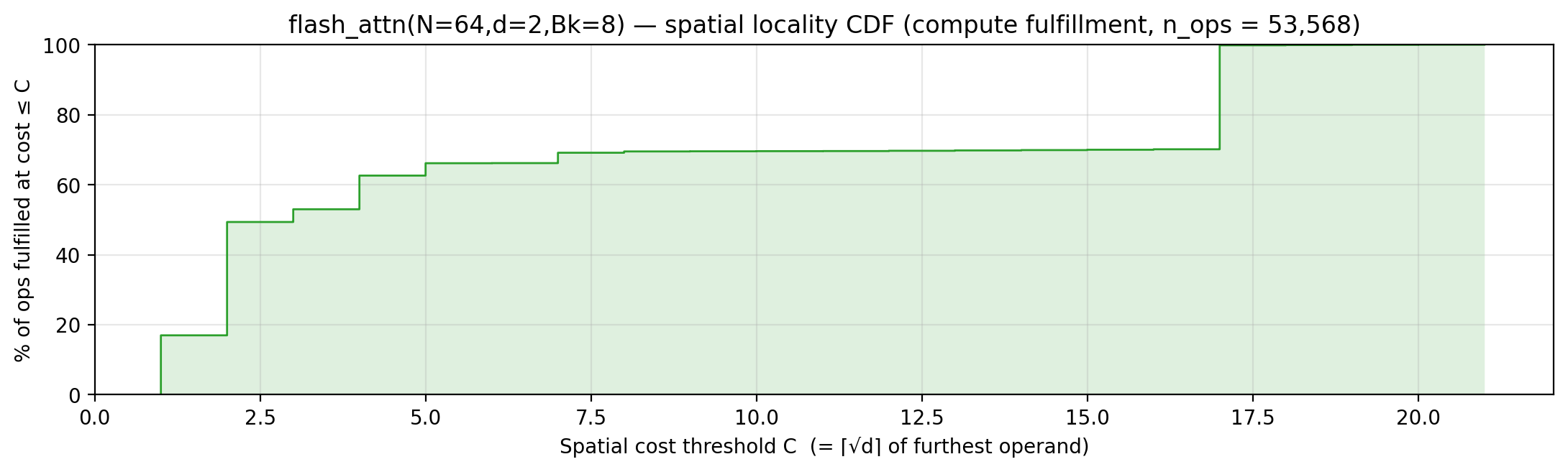
Spatial locality CDF — compute-fulfillment as a function of radius.
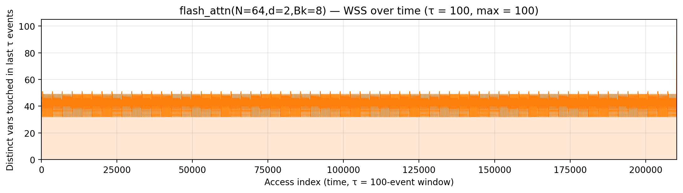
Working-set size over a τ = 100-event window (max = 100).
matvec_row (code)
n=64. Algorithm. y[i] = Σ_j A[i][j] · x[j], outer loop over i.
A is read row-major (contiguous); x is re-read n times.
Manual placement. The Python signature matvec(A, x) puts x at
the end of the arg stack (addrs n²+1..n²+n). Each x[j] is re-read
n times — from those high arg addresses. Preloading x once into a
c_X scratch buffer at the bottom of the stack cuts every subsequent
x access to near-top-of-scratch cost:
s, tmp (addrs 1-2) — accumulator + tmp
c_X (addrs 3..n+2) — hot x buffer (one-time arg preload)
y (addrs n+3..2n+2) — output
Drops manual from 455,587 to 218,552 (−52%), now within 2 % of
global_density (213,783).
Theoretical floor for n=64 matvec (applies to all three variants below): gemini/optimal-matvec.md derives a strict lower bound under the semi-ring + polyhedron restrictions: the compulsory-I/O barrier is 180,960 (just the arg transport cost), and the achievable minimum is 208,832.
matvec_blocked(below) now implements the exact schedule prescribed by the doc and lands at 208,832 — the floor itself.matvec_row(218,552, +5%) andmatvec_col(217,952, +4%) are close but pay for their simpler layouts.
Working-set size over time (peak = 128).
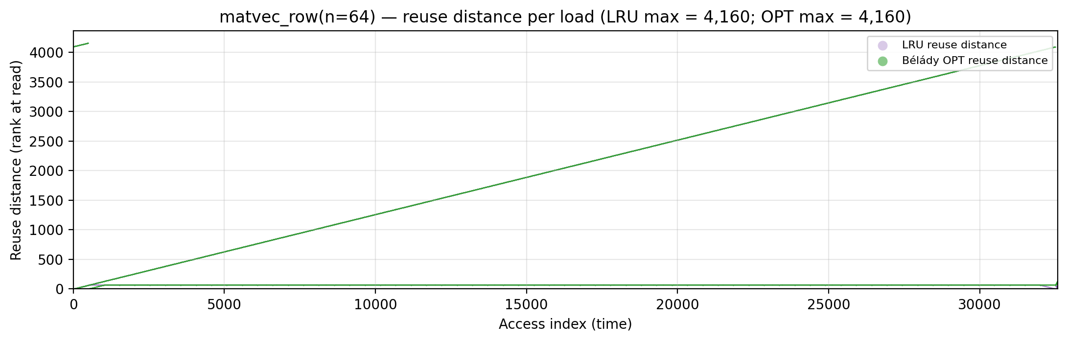
Reuse distance per load — LRU vs Bélády OPT (max LRU = 4,160; max OPT = 4,160).
Miss-ratio curve — LRU vs Bélády OPT misses by cache capacity.
Per-tick TU LP floor — integrand of global_density: Σ_i ρ_{(i)} · √i over currently-live vars, ranked by density; the area equals global_density.
Per-tick splitting LP floor — integrand of local_density: Σ_i ρ_{(i)} · √i over the currently-active per-burst virtual intervals; the area equals the geometric portion of local_density.
Per-tick polymatroid LP floor — integrand of polymatroid_lb: Σ_v reads_v · ⌈√d_v⌉ / lifespan(v) over live vars, where d_v is each variable’s LP-implied static depth (gemini/polymatroid-relaxation.md). The area equals the geometric portion of polymatroid_lb.
Rolling spatial intensity — heartbeat plot of ops / Σ ⌈√d⌉ over a sliding window.
Cumulative compute vs fetch cost — slope = instantaneous spatial arithmetic intensity.
Gravity well — per-load fetch-cost ⌈√d⌉ scatter.
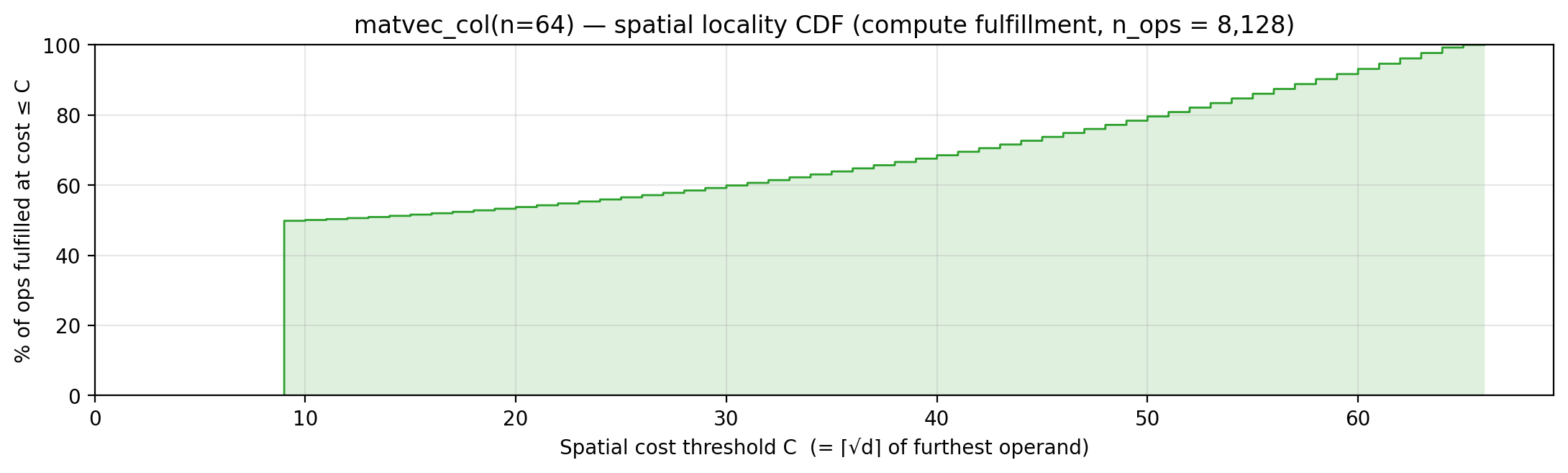
Spatial locality CDF — compute-fulfillment as a function of radius.
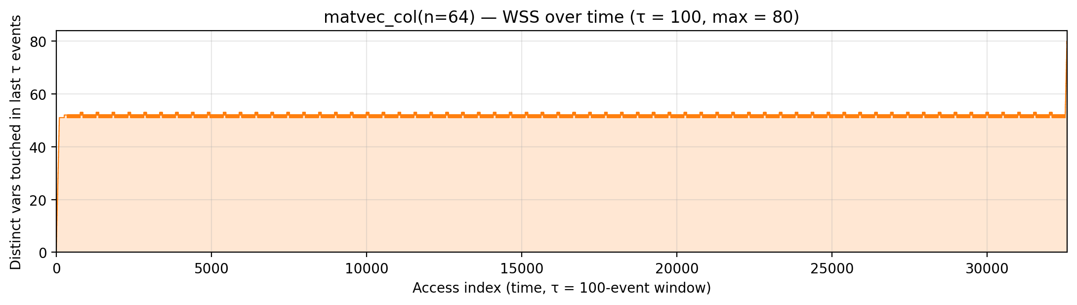
Working-set size over a τ = 2,529-event window (max = 1,052).
matvec_col (code)
n=64. Algorithm. Outer loop over j: for each column of A, fold
A[i][j] · x[j] into y[i]. A is read column-major (strided by n).
Manual placement. Same as row-major: tmp, y, x hot at 1..2n+1; A
cold at 2n+2.. . Column-major read pattern spreads A accesses across
the whole bulk region in stride-n jumps, which bytedmd_live rewards
(177k vs row’s 229k) but manual barely distinguishes (212k vs 238k) —
again, the sum is fixed.
Working-set size over time (peak = 66).
Reuse distance per load — LRU vs Bélády OPT (max LRU = 4,160; max OPT = 4,160).
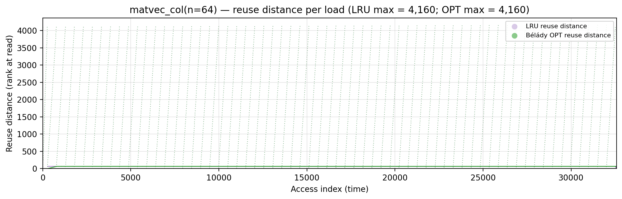
Miss-ratio curve — LRU vs Bélády OPT misses by cache capacity.
Per-tick TU LP floor — integrand of global_density: Σ_i ρ_{(i)} · √i over currently-live vars, ranked by density; the area equals global_density.
Per-tick splitting LP floor — integrand of local_density: Σ_i ρ_{(i)} · √i over the currently-active per-burst virtual intervals; the area equals the geometric portion of local_density.
Per-tick polymatroid LP floor — integrand of polymatroid_lb: Σ_v reads_v · ⌈√d_v⌉ / lifespan(v) over live vars, where d_v is each variable’s LP-implied static depth (gemini/polymatroid-relaxation.md). The area equals the geometric portion of polymatroid_lb.
Rolling spatial intensity — heartbeat plot of ops / Σ ⌈√d⌉ over a sliding window.
Cumulative compute vs fetch cost — slope = instantaneous spatial arithmetic intensity.
Gravity well — per-load fetch-cost ⌈√d⌉ scatter.
Spatial locality CDF — compute-fulfillment as a function of radius.
Working-set size over a τ = 2,529-event window (max = 1,019).
matvec_blocked (code)
n=64, B=8. Algorithm. Stationary-Accumulator 1D-Blocked MatVec
(gemini/optimal-matvec.md). Outer
loop iterates over 8-column blocks of x. For each block, load the
current 8 x-values once into a tight L1 cache, then sweep every row
of A through a single scalar accumulator s, flushing the
partial sum back to y[i] after each row. Subsequent x-blocks
reload the partial sum from y[i], add their contribution, and
store back.
Manual placement. Addresses laid out strictly by access
frequency:
s (addr 1) — stationary accumulator (4,096 MACs)
tmp (addr 2) — multiply intermediate (4,032 reads)
c_x (addrs 3..10) — current 8-element x-block cache
y (addrs 11..74) — output / partial-sum array
Inner loop footprint is strictly addrs 1..10 — everything hotter than the output array sits in a register-file-sized window. Under the semi-ring restriction the full argument-transport cost (A=176,800 + x=4,160 = 180,960) is unavoidable; the remainder (27,872 of L1 reads, y-flushes, and epilogue) is what the optimal schedule minimises.
Manual lands at 208,832 — the provable floor for n=64 matvec
under the semi-ring + polyhedron restrictions (doc §2). Every
other schedule in this family either reloads x from the deep arg
stack (paying 4,160 per row), stretches the scratch footprint
past addr 10 (inflating every inner-loop read), or wastes cycles
pulling A through a cached tile it cannot reuse. This hits every
term of the doc’s exact breakdown:
| term | cost |
|---|---|
| A arg sweep (4,096 reads) | 176,800 |
| x arg sweep (64 reads) | 4,160 |
| c_x reads (4,096 × avg 2.875) | 11,776 |
| s + tmp inner reads (4,032 × 3) | 12,096 |
| y flush-and-reload (7 × 436) | 3,052 |
| s-store overhead (512 touches) | 512 |
| output epilogue | 436 |
| total | 208,832 |
Working-set size over time (peak = 129).
Reuse distance per load — LRU vs Bélády OPT (max LRU = 4,160; max OPT = 4,160).
Miss-ratio curve — LRU vs Bélády OPT misses by cache capacity.
Per-tick TU LP floor — integrand of global_density: Σ_i ρ_{(i)} · √i over currently-live vars, ranked by density; the area equals global_density.
Per-tick splitting LP floor — integrand of local_density: Σ_i ρ_{(i)} · √i over the currently-active per-burst virtual intervals; the area equals the geometric portion of local_density.
Per-tick polymatroid LP floor — integrand of polymatroid_lb: Σ_v reads_v · ⌈√d_v⌉ / lifespan(v) over live vars, where d_v is each variable’s LP-implied static depth (gemini/polymatroid-relaxation.md). The area equals the geometric portion of polymatroid_lb.

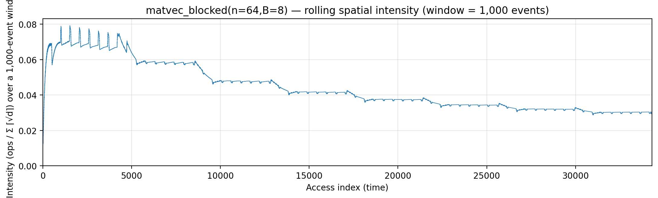
Rolling spatial intensity — heartbeat plot of ops / Σ ⌈√d⌉ over a sliding window.
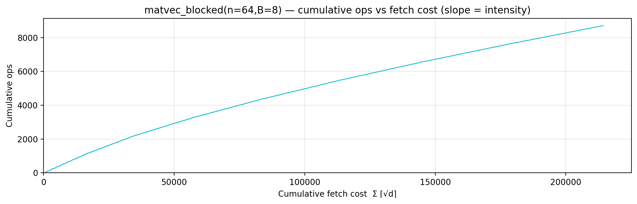
Cumulative compute vs fetch cost — slope = instantaneous spatial arithmetic intensity.
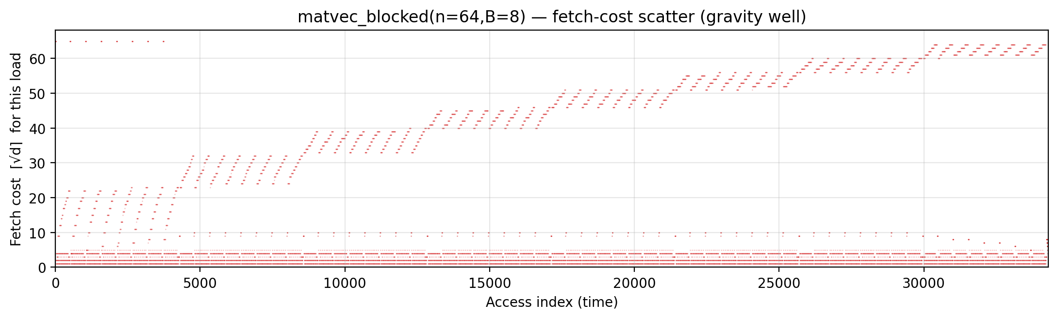
Gravity well — per-load fetch-cost ⌈√d⌉ scatter.
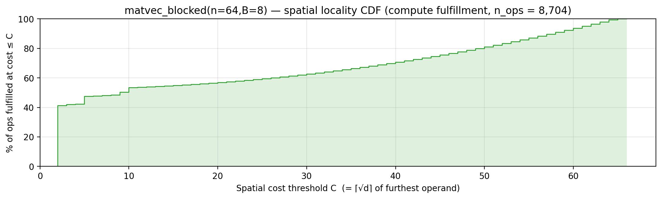
Spatial locality CDF — compute-fulfillment as a function of radius.
Working-set size over a τ = 100-event window (max = 82).
fft_iterative (code)
N=256. Algorithm. In-place iterative radix-2 Cooley–Tukey:
bit-reverse permutation followed by log₂N = 8 stages of N/2 butterflies
each. Real twiddle stand-in (the ByteDMD cost depends only on the
load pattern).
Manual placement. Single N-slot array x at addrs 1..N — the entire
working set lives in the hot region. No temps, no recursion, no bulk
data region. Manual cost (25,528) is well below bytedmd_live
(44,212) — a cheap-placement win that recency heuristics can’t
anticipate once the working set fits entirely at low addresses.
Working-set size over time (peak = 257).
Reuse distance per load — LRU vs Bélády OPT (max LRU = 256; max OPT = 256).
Miss-ratio curve — LRU vs Bélády OPT misses by cache capacity.
Per-tick TU LP floor — integrand of global_density: Σ_i ρ_{(i)} · √i over currently-live vars, ranked by density; the area equals global_density.
Per-tick splitting LP floor — integrand of local_density: Σ_i ρ_{(i)} · √i over the currently-active per-burst virtual intervals; the area equals the geometric portion of local_density.
Per-tick polymatroid LP floor — integrand of polymatroid_lb: Σ_v reads_v · ⌈√d_v⌉ / lifespan(v) over live vars, where d_v is each variable’s LP-implied static depth (gemini/polymatroid-relaxation.md). The area equals the geometric portion of polymatroid_lb.
Rolling spatial intensity — heartbeat plot of ops / Σ ⌈√d⌉ over a sliding window.
Cumulative compute vs fetch cost — slope = instantaneous spatial arithmetic intensity.
Gravity well — per-load fetch-cost ⌈√d⌉ scatter.
Spatial locality CDF — compute-fulfillment as a function of radius.
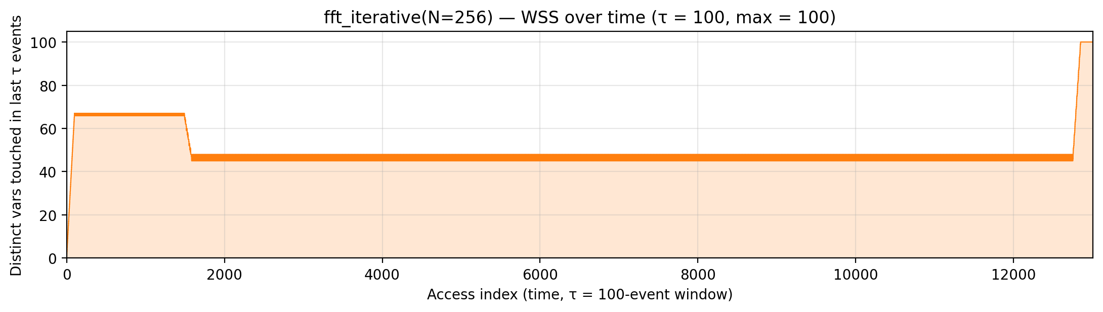
Working-set size over a τ = 256-event window (max = 256).
fft_recursive (code)
N=256. Algorithm. In-place recursive radix-2 Cooley–Tukey:
split into even/odd halves, recurse, then combine with twiddles.
Manual placement. A single x[1..N] working buffer on scratch;
the recursion carries a logical stride so leaves route arg-stack
cells directly into their bit-reversed scratch slots without any
intermediate copy. Every butterfly then operates purely in-place.
Peak scratch footprint is exactly N and every read pays
⌈√addr⌉ over addrs 1..N only. The resulting manual cost (28,560)
is the mathematical minimum under this model: log₂N + 2 = 10
sequential passes over N cells (1 arg-load leaf pass + log₂N = 8
butterfly passes + 1 output epilogue), and it even beats
bytedmd_live (33,110).
Working-set size over time (peak = 257).
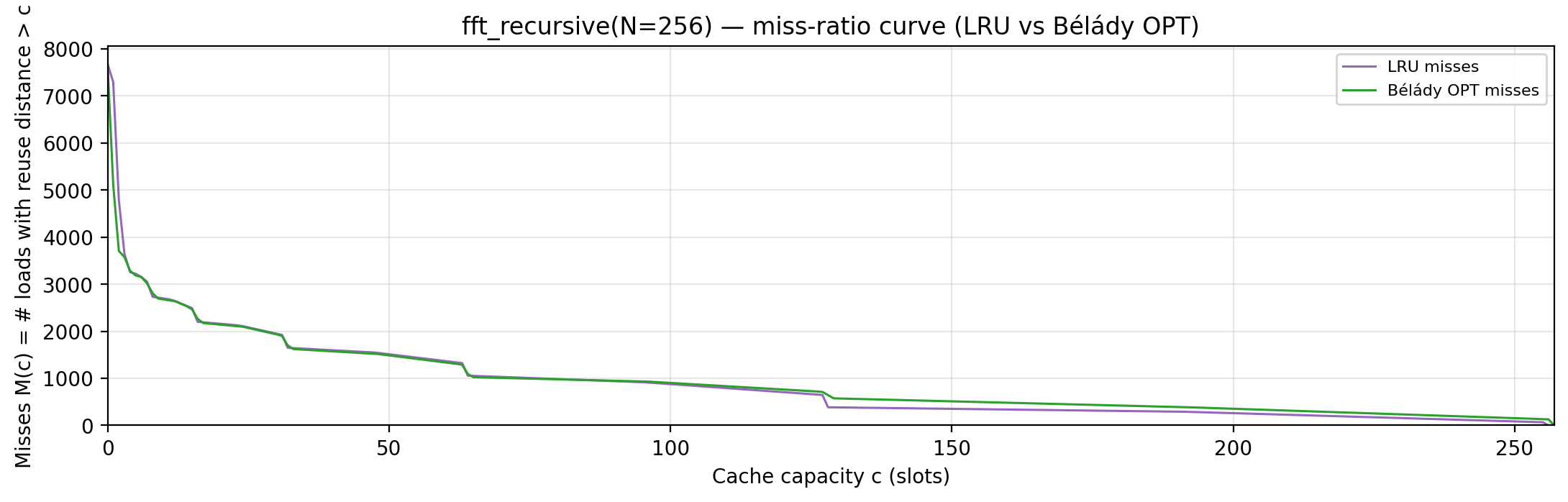
Reuse distance per load — LRU vs Bélády OPT (max LRU = 256; max OPT = 256).
Miss-ratio curve — LRU vs Bélády OPT misses by cache capacity.
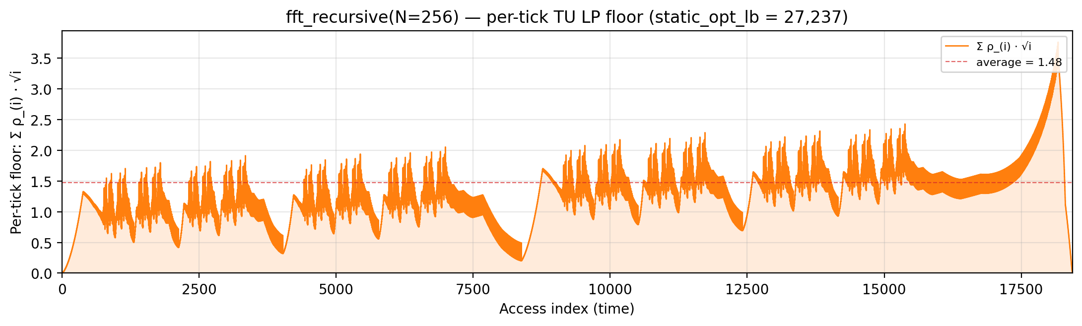
Per-tick TU LP floor — integrand of global_density: Σ_i ρ_{(i)} · √i over currently-live vars, ranked by density; the area equals global_density.
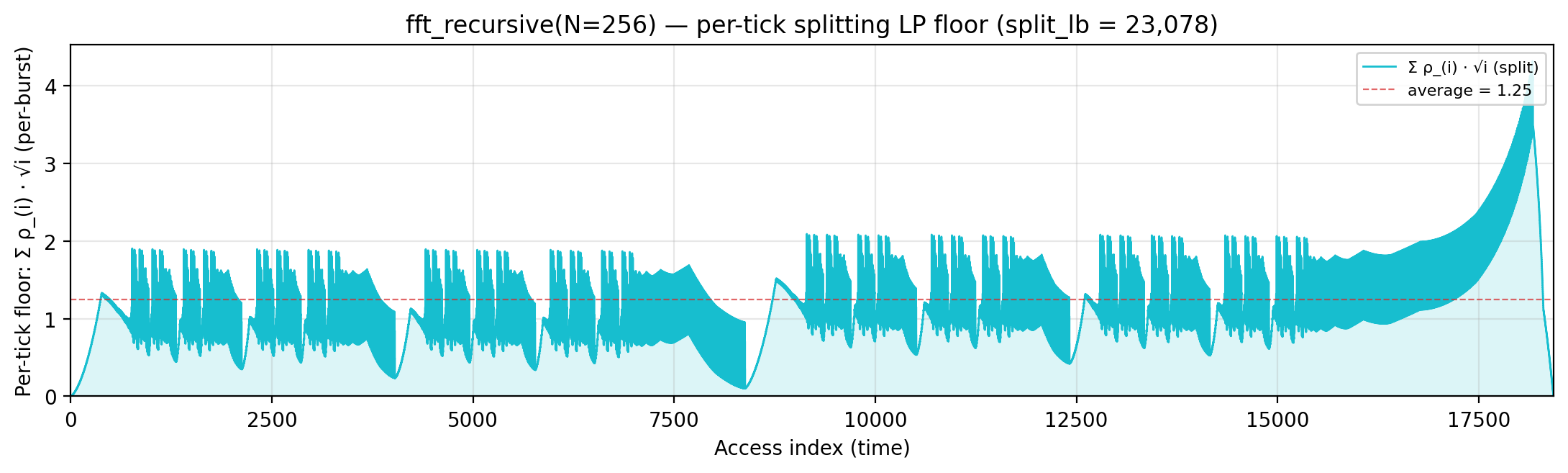
Per-tick splitting LP floor — integrand of local_density: Σ_i ρ_{(i)} · √i over the currently-active per-burst virtual intervals; the area equals the geometric portion of local_density.
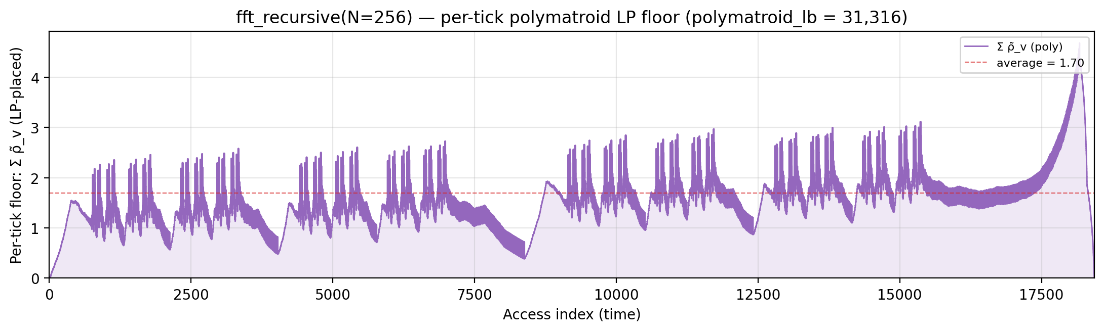
Per-tick polymatroid LP floor — integrand of polymatroid_lb: Σ_v reads_v · ⌈√d_v⌉ / lifespan(v) over live vars, where d_v is each variable’s LP-implied static depth (gemini/polymatroid-relaxation.md). The area equals the geometric portion of polymatroid_lb.
Rolling spatial intensity — heartbeat plot of ops / Σ ⌈√d⌉ over a sliding window.
Cumulative compute vs fetch cost — slope = instantaneous spatial arithmetic intensity.
Gravity well — per-load fetch-cost ⌈√d⌉ scatter.
Spatial locality CDF — compute-fulfillment as a function of radius.
Working-set size over a τ = 113-event window (max = 113).
stencil_naive (code)
32×32, one sweep. Algorithm. 5-point Jacobi row-major sweep:
B[i][j] = 0.2 · (A[i][j] + A[i±1][j] + A[i][j±1]) for interior cells.
Manual placement. Rolling 3-row buffer at addrs 1..3n: each A cell is read exactly once from the arg stack (streaming preload, one row at a time) and all 5 stencil reads hit the rolling buffer at low addresses. B sits at addrs 3n+1..3n+n².
r0, r1, r2 (addrs 1..3n) — rotated via (i-1)%3, i%3, (i+1)%3
B (addrs 3n+1..) — output matrix
Drops manual from 121,628 to 78,968 (−35%).
Working-set size over time (peak = 930).
Reuse distance per load — LRU vs Bélády OPT (max LRU = 1,023; max OPT = 1,023).
Miss-ratio curve — LRU vs Bélády OPT misses by cache capacity.
Per-tick TU LP floor — integrand of global_density: Σ_i ρ_{(i)} · √i over currently-live vars, ranked by density; the area equals global_density.
Per-tick splitting LP floor — integrand of local_density: Σ_i ρ_{(i)} · √i over the currently-active per-burst virtual intervals; the area equals the geometric portion of local_density.
Per-tick polymatroid LP floor — integrand of polymatroid_lb: Σ_v reads_v · ⌈√d_v⌉ / lifespan(v) over live vars, where d_v is each variable’s LP-implied static depth (gemini/polymatroid-relaxation.md). The area equals the geometric portion of polymatroid_lb.
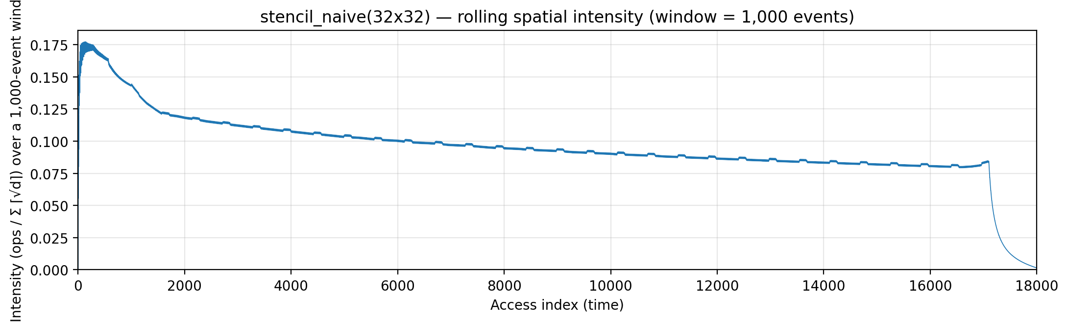
Rolling spatial intensity — heartbeat plot of ops / Σ ⌈√d⌉ over a sliding window.
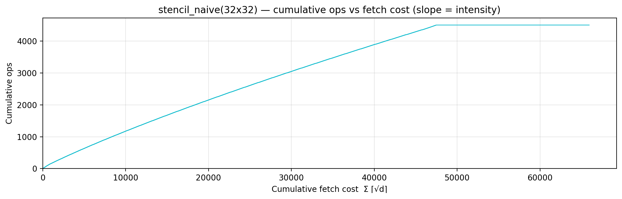
Cumulative compute vs fetch cost — slope = instantaneous spatial arithmetic intensity.
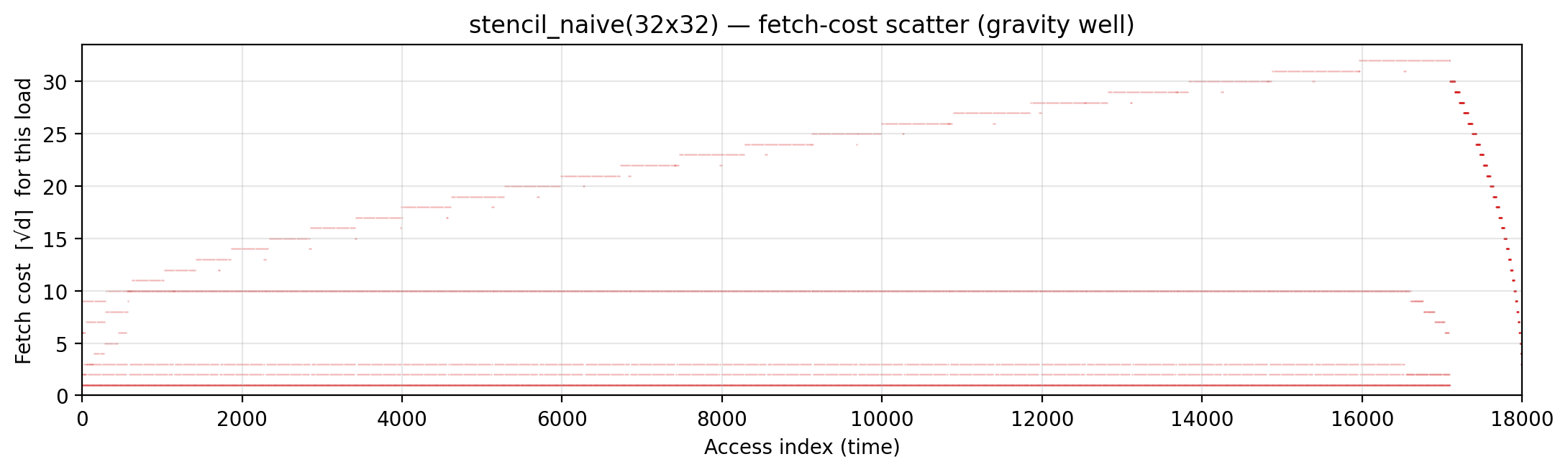
Gravity well — per-load fetch-cost ⌈√d⌉ scatter.
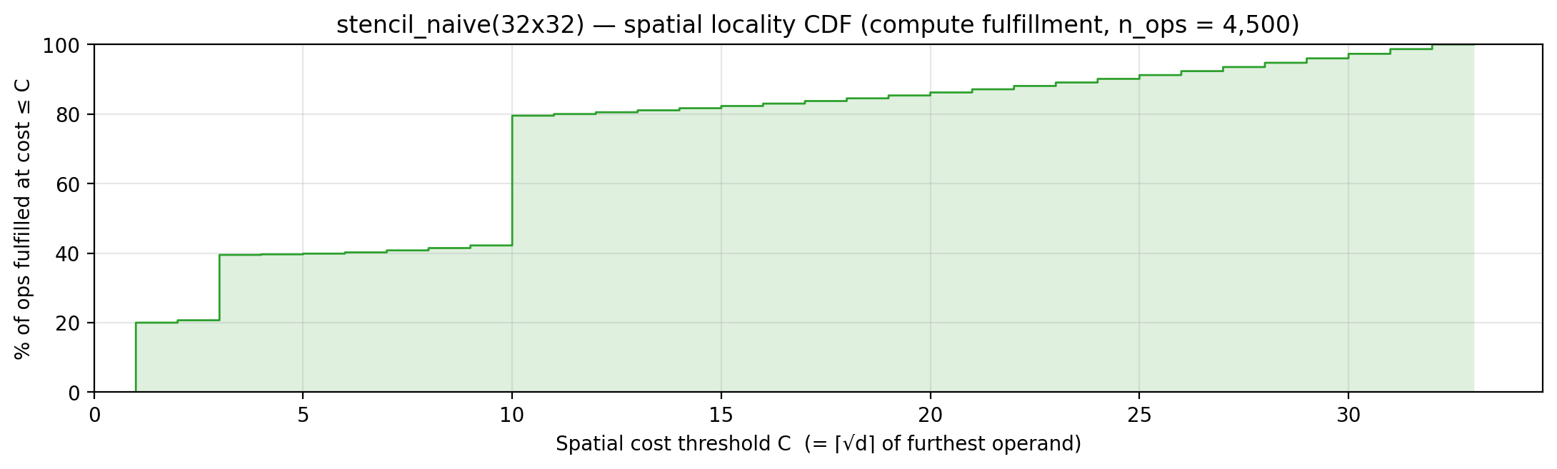
Spatial locality CDF — compute-fulfillment as a function of radius.
Working-set size over a τ = 512-event window (max = 512).
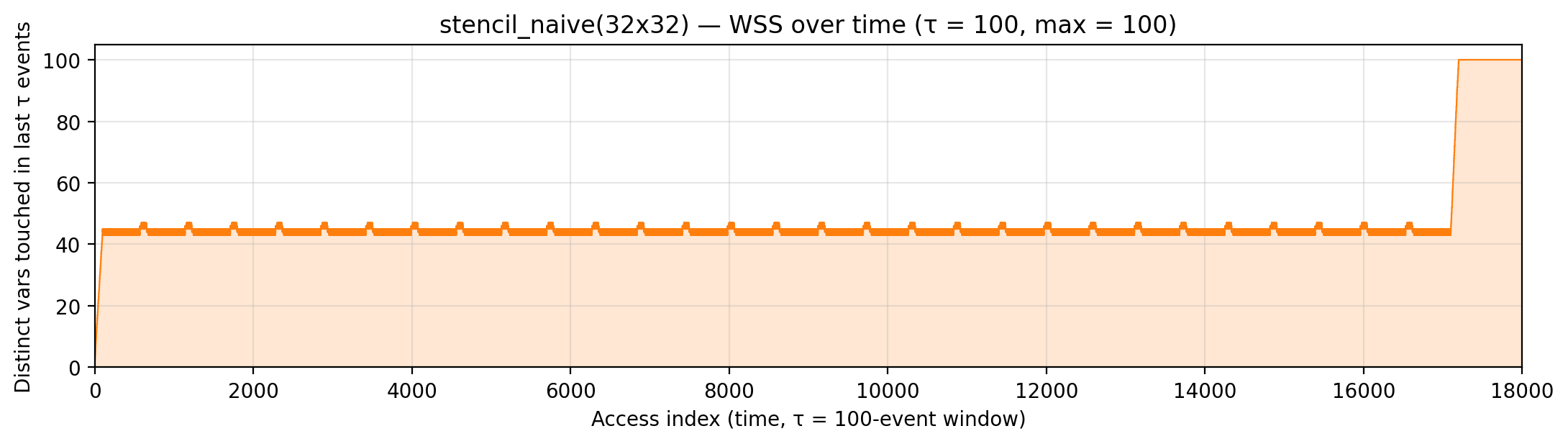
stencil_recursive (code)
32×32, one sweep, leaf=8. Algorithm. Quad-tree split of the 2D
domain, naive sweep at leaf tiles of size 8×8. (Trapezoidal
cache-oblivious stencil is not implemented — that form requires a time
dimension.)
Manual placement. Same A, B layout as naive. Manual cost is
identical to naive (99,276) because every A cell is still touched
exactly 5× — the cost sum Σ⌈√addr⌉ is invariant to access order.
bytedmd_live distinguishes them (37,737 vs 44,468) via recency
effects only.
Working-set size over time (peak = 908).
Reuse distance per load — LRU vs Bélády OPT (max LRU = 1,023; max OPT = 1,023).
Miss-ratio curve — LRU vs Bélády OPT misses by cache capacity.
Per-tick TU LP floor — integrand of global_density: Σ_i ρ_{(i)} · √i over currently-live vars, ranked by density; the area equals global_density.
Per-tick splitting LP floor — integrand of local_density: Σ_i ρ_{(i)} · √i over the currently-active per-burst virtual intervals; the area equals the geometric portion of local_density.
Per-tick polymatroid LP floor — integrand of polymatroid_lb: Σ_v reads_v · ⌈√d_v⌉ / lifespan(v) over live vars, where d_v is each variable’s LP-implied static depth (gemini/polymatroid-relaxation.md). The area equals the geometric portion of polymatroid_lb.
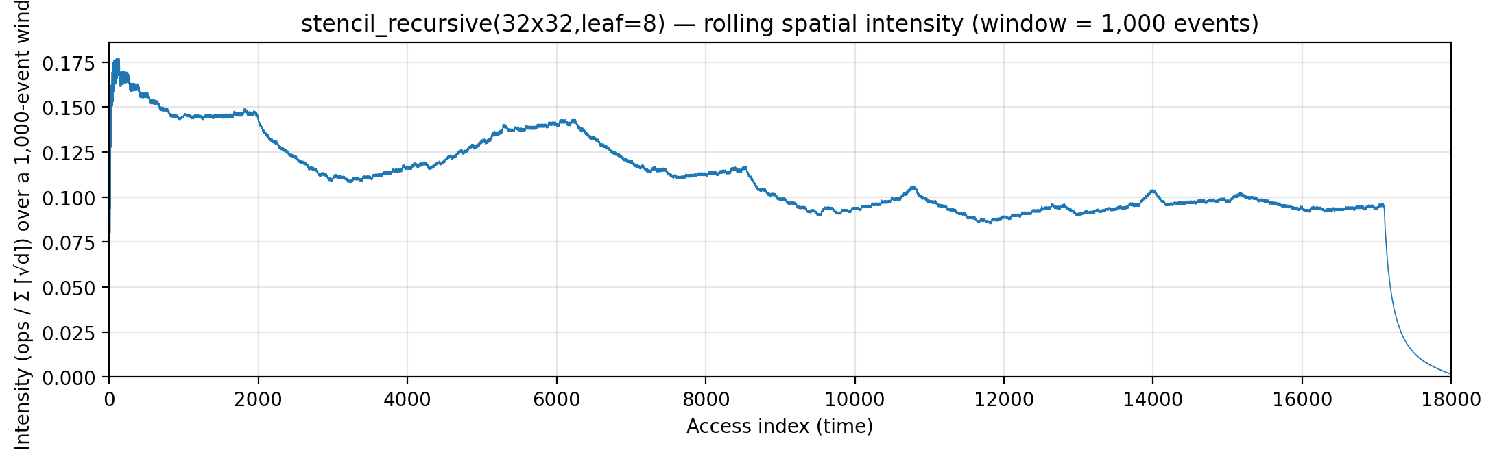
Rolling spatial intensity — heartbeat plot of ops / Σ ⌈√d⌉ over a sliding window.
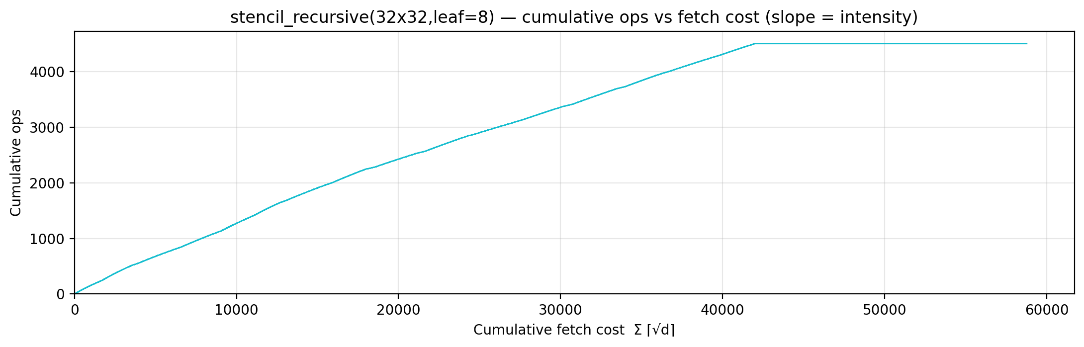
Cumulative compute vs fetch cost — slope = instantaneous spatial arithmetic intensity.
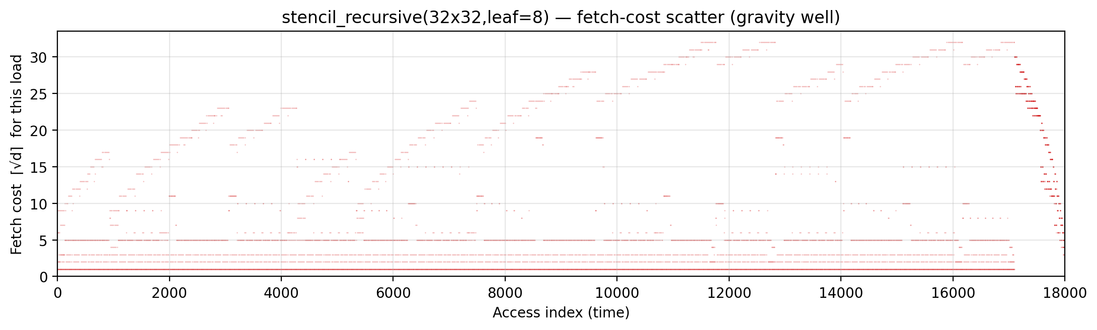
Gravity well — per-load fetch-cost ⌈√d⌉ scatter.
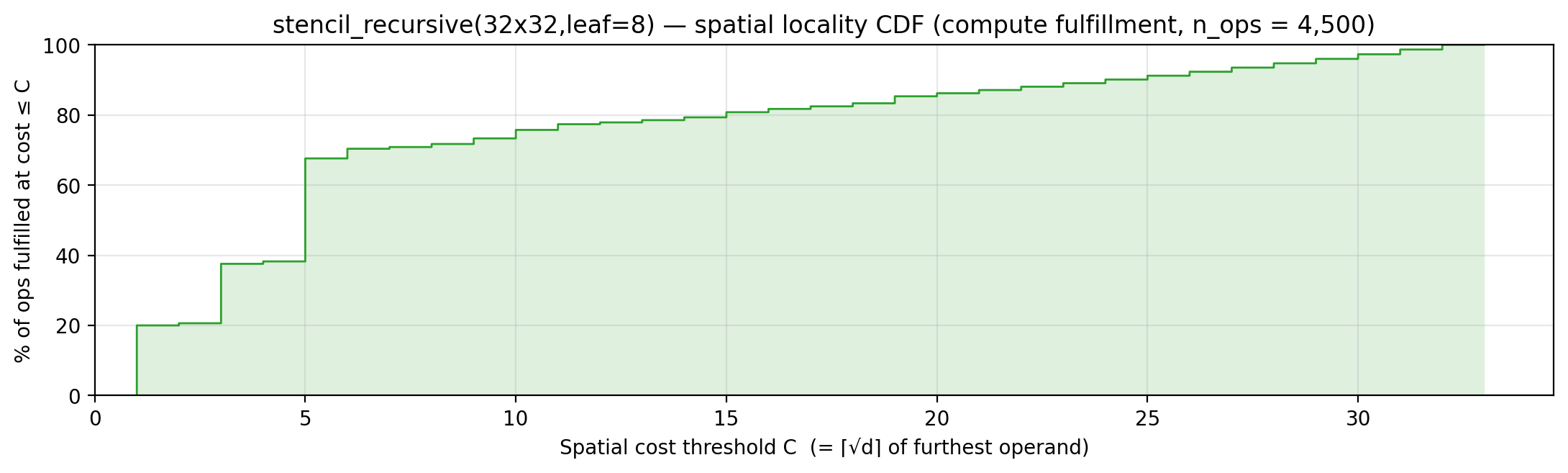
Spatial locality CDF — compute-fulfillment as a function of radius.
Working-set size over a τ = 492-event window (max = 492).
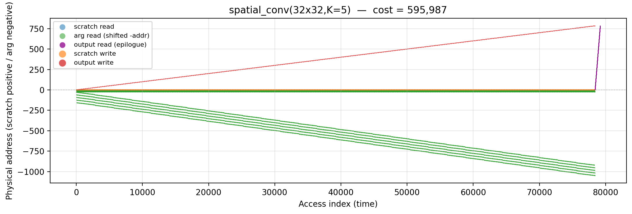
spatial_conv (code)
32×32, K=5. Algorithm. Single-channel 2D convolution:
O[i][j] = Σ_{ki,kj} A[i+ki][j+kj] · W[ki][kj]. Output is 28×28.
Manual placement. Scalar s at addr 1, K² = 25-slot kernel W at
2..26 (hot, reused for every output cell), H·W image at 27.. (cold
bulk). Each output cell reads s once then touches image and kernel
K² times.
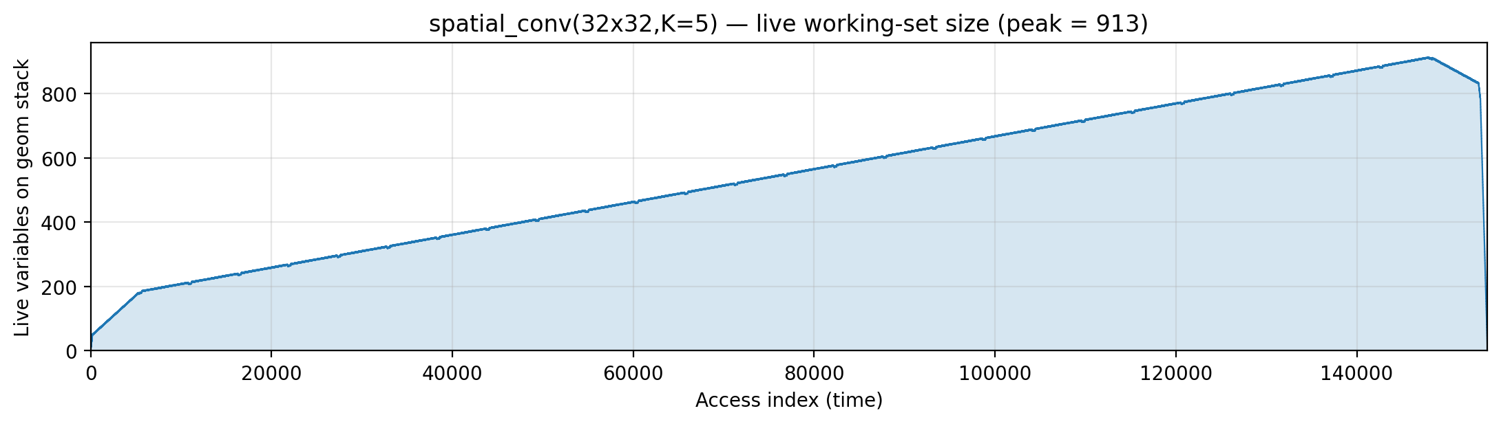
Working-set size over time (peak = 913).
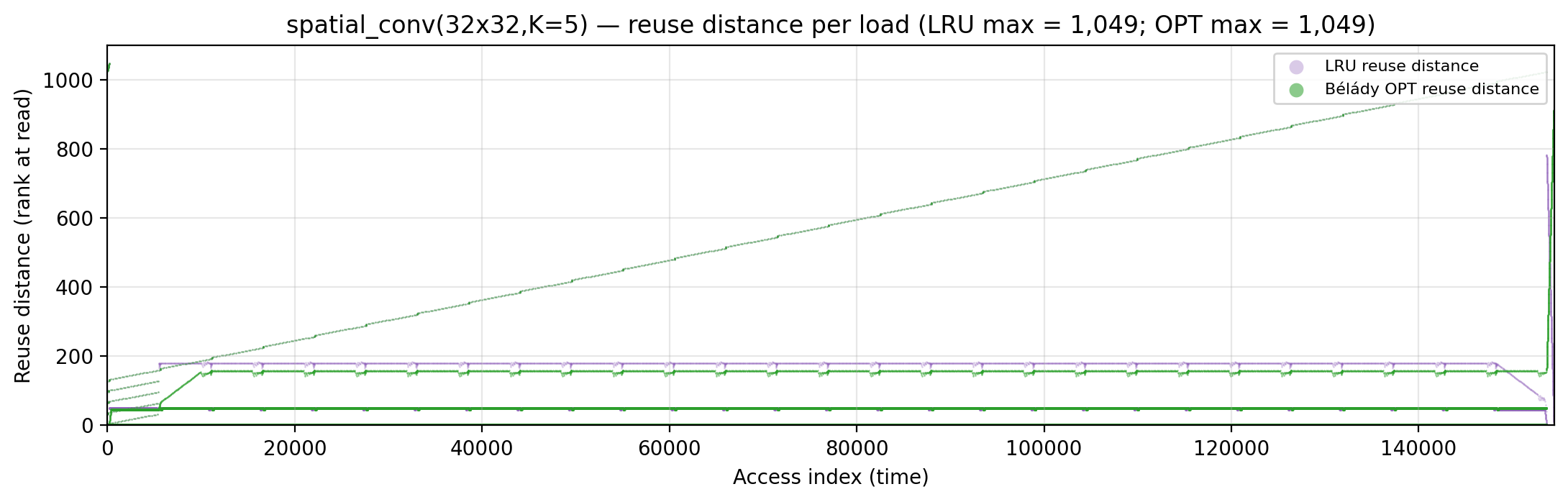
Reuse distance per load — LRU vs Bélády OPT (max LRU = 1,049; max OPT = 1,049).
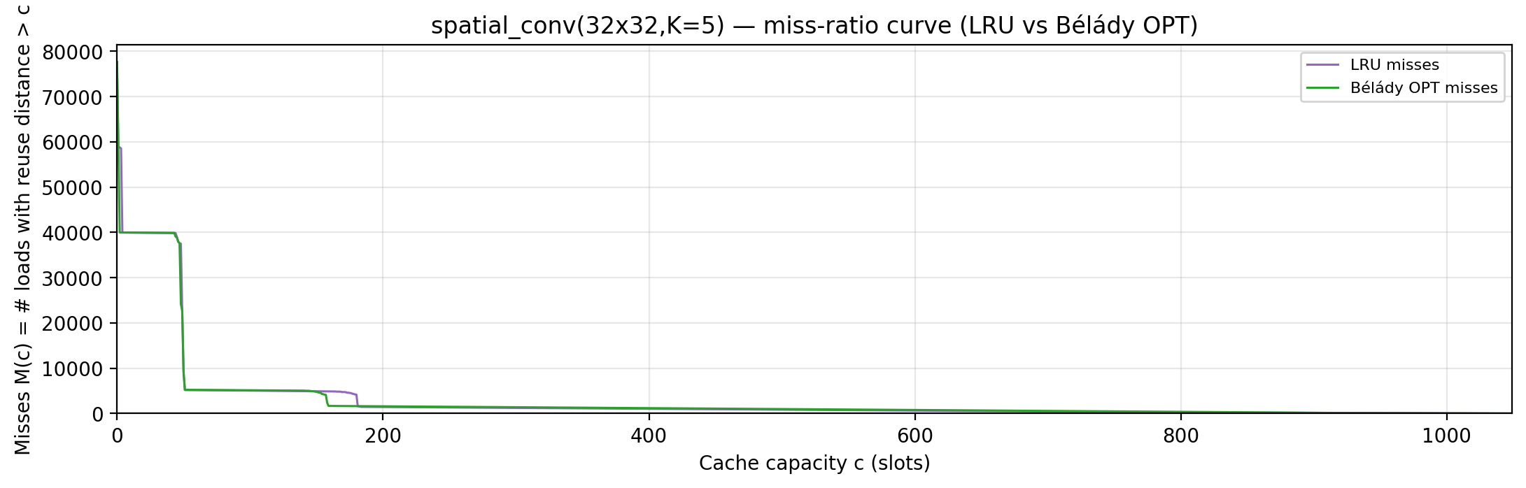
Miss-ratio curve — LRU vs Bélády OPT misses by cache capacity.
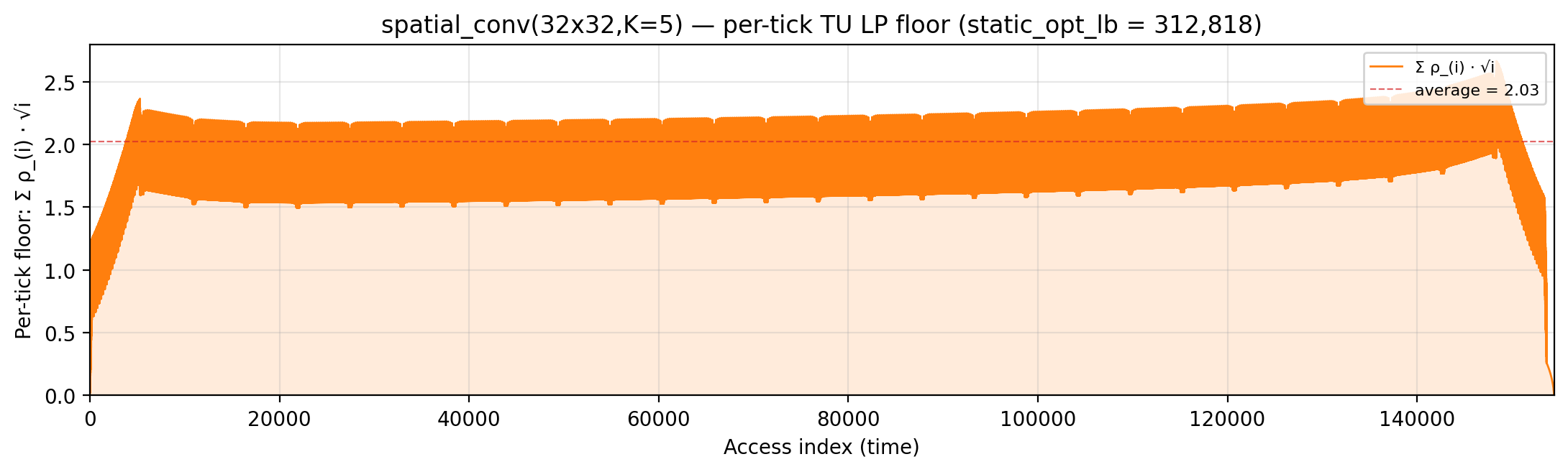
Per-tick TU LP floor — integrand of global_density: Σ_i ρ_{(i)} · √i over currently-live vars, ranked by density; the area equals global_density.
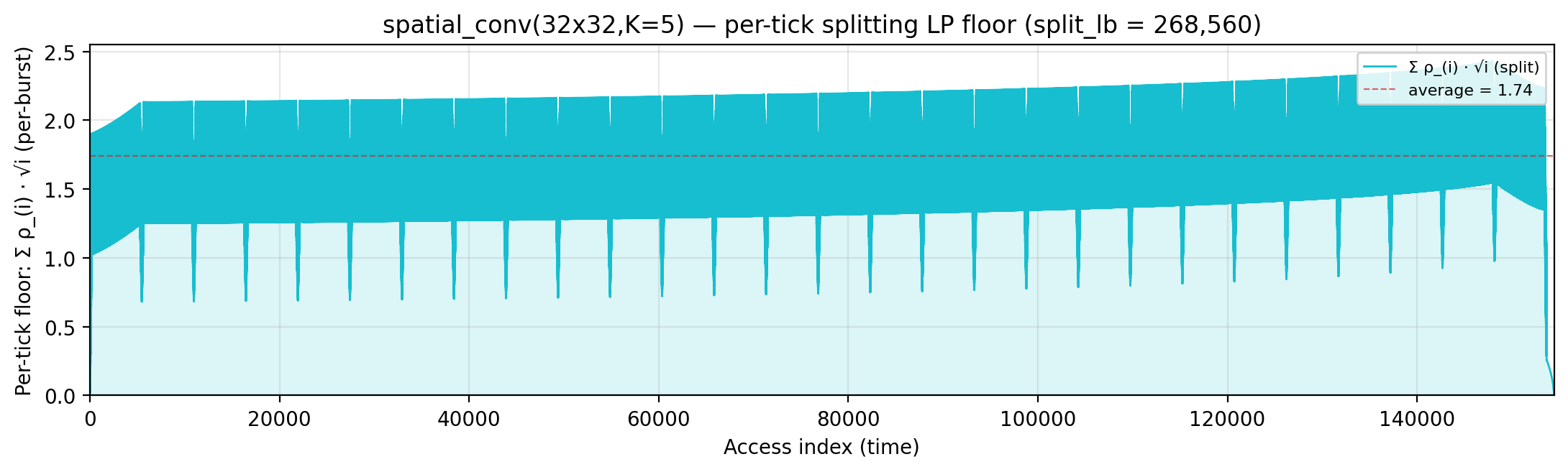
Per-tick splitting LP floor — integrand of local_density: Σ_i ρ_{(i)} · √i over the currently-active per-burst virtual intervals; the area equals the geometric portion of local_density.
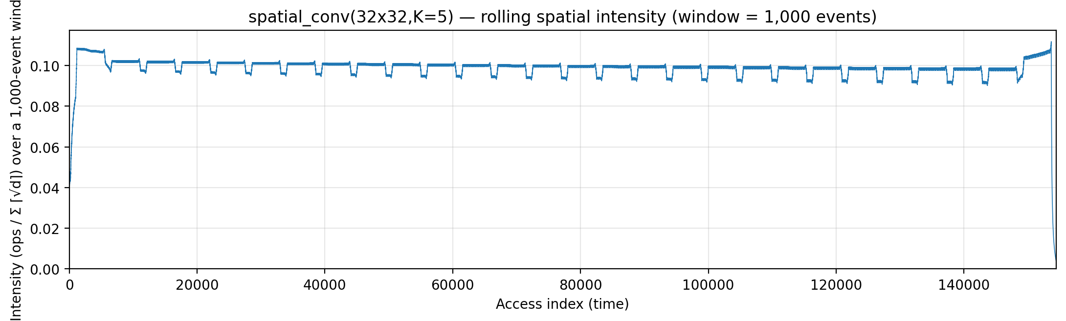
Rolling spatial intensity — heartbeat plot of ops / Σ ⌈√d⌉ over a sliding window.
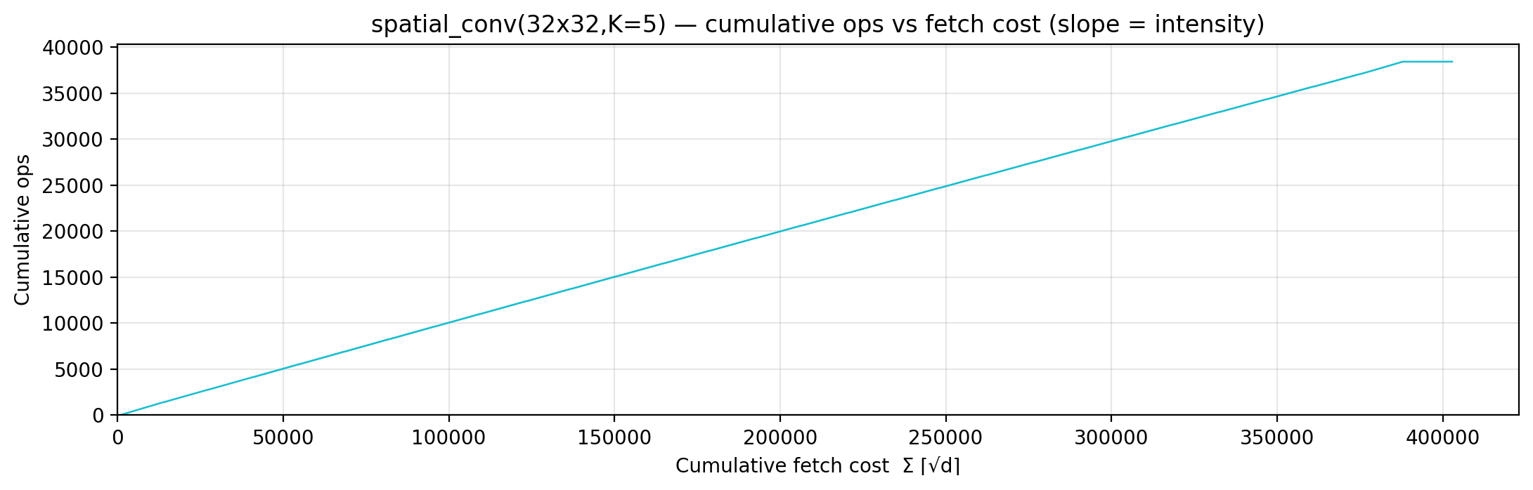
Cumulative compute vs fetch cost — slope = instantaneous spatial arithmetic intensity.
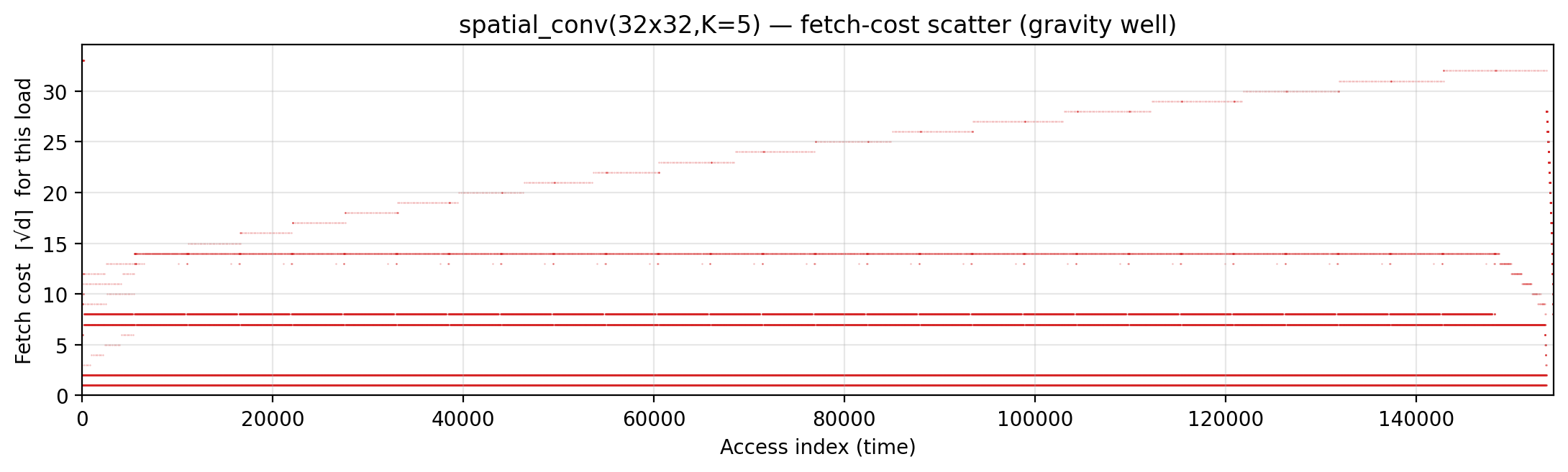
Gravity well — per-load fetch-cost ⌈√d⌉ scatter.
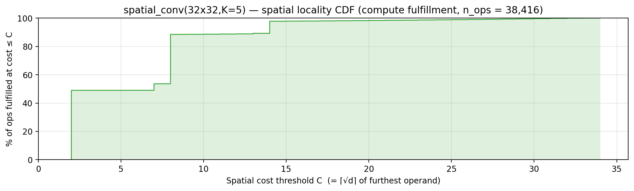
Spatial locality CDF — compute-fulfillment as a function of radius.
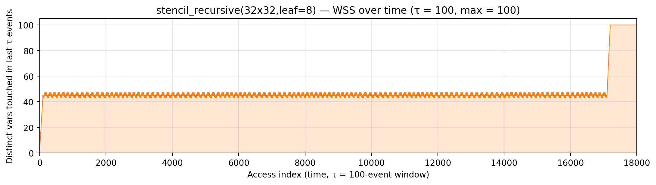
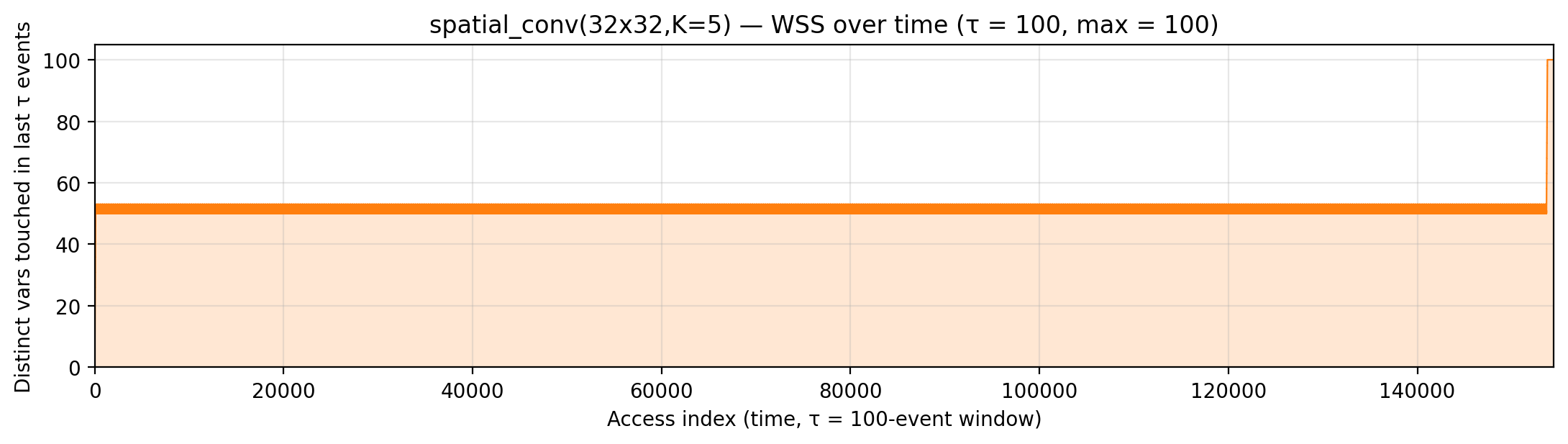
Working-set size over a τ = 51-event window (max = 51).
regular_conv (code)
16×16, K=3, Cin=4, Cout=4. Algorithm. Full multi-channel CNN
layer: O[i][j][co] = Σ_{ki,kj,ci} A[i+ki][j+kj][ci] · W[ki][kj][ci][co].
Manual placement. Scalar s, then K²·Cin·Cout = 144-slot kernel
(channel pairs inner-most), then H·W·Cin image (channel inner-most).
Kernel fits in the hot region so all 144 weights are cheap; image
sweeps the mid-range bulk for each of the Cin channels per spatial
position.
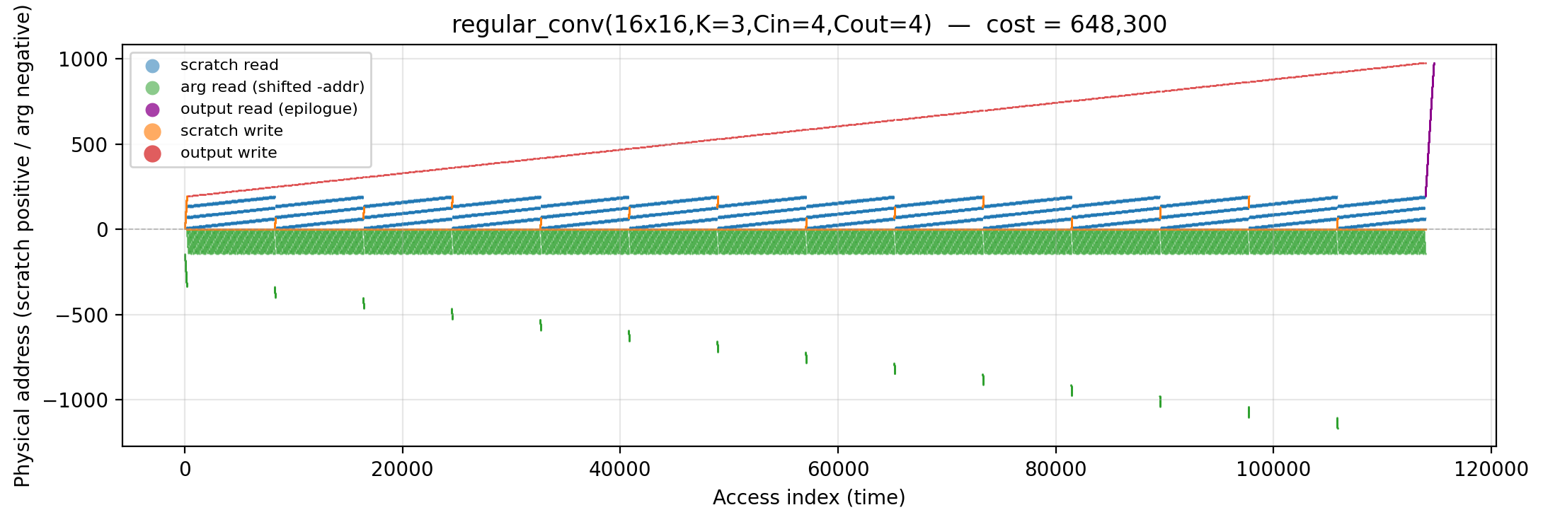
Working-set size over time (peak = 1,016).

Reuse distance per load — LRU vs Bélády OPT (max LRU = 1,168; max OPT = 1,168).
Miss-ratio curve — LRU vs Bélády OPT misses by cache capacity.
Per-tick TU LP floor — integrand of global_density: Σ_i ρ_{(i)} · √i over currently-live vars, ranked by density; the area equals global_density.

Per-tick splitting LP floor — integrand of local_density: Σ_i ρ_{(i)} · √i over the currently-active per-burst virtual intervals; the area equals the geometric portion of local_density.

Rolling spatial intensity — heartbeat plot of ops / Σ ⌈√d⌉ over a sliding window.
Cumulative compute vs fetch cost — slope = instantaneous spatial arithmetic intensity.

Gravity well — per-load fetch-cost ⌈√d⌉ scatter.
Spatial locality CDF — compute-fulfillment as a function of radius.
Working-set size over a τ = 193-event window (max = 193).
fft_conv (code)
N=256. Algorithm. 1D circular convolution via FFT:
IFFT(FFT(x) · FFT(y)). Two forward FFTs, an N-element pointwise
multiply, and one inverse FFT.
Manual placement. Four stacked optimizations
(gemini/optimize-fft-conv.md):
(1) 2D L1 cache blocking — factor the 256-point FFT into 16×16 row
and column passes so every butterfly runs inside a 16-cell
cache_A at addrs 1..16. (2) Shared workspace — only two
N-sized buffers instead of three; X is reused across FFT(X),
FFT(Y), and IFFT(Z). (3) Fused bit-reversal — arg-stack inputs
map directly into their bit-reversed coordinates on first touch
(no explicit permutation pass). (4) Fused pointwise Z — the
IFFT’s cache-load step reads X_fft[rev_idx] * Y_fft[rev_idx]
on-the-fly, skipping a materialized Z array. Together these drop
manual 273,318 → 91,922 (−66 %), cheaper than bytedmd_live
(148,641) but still above global_density (57,400).
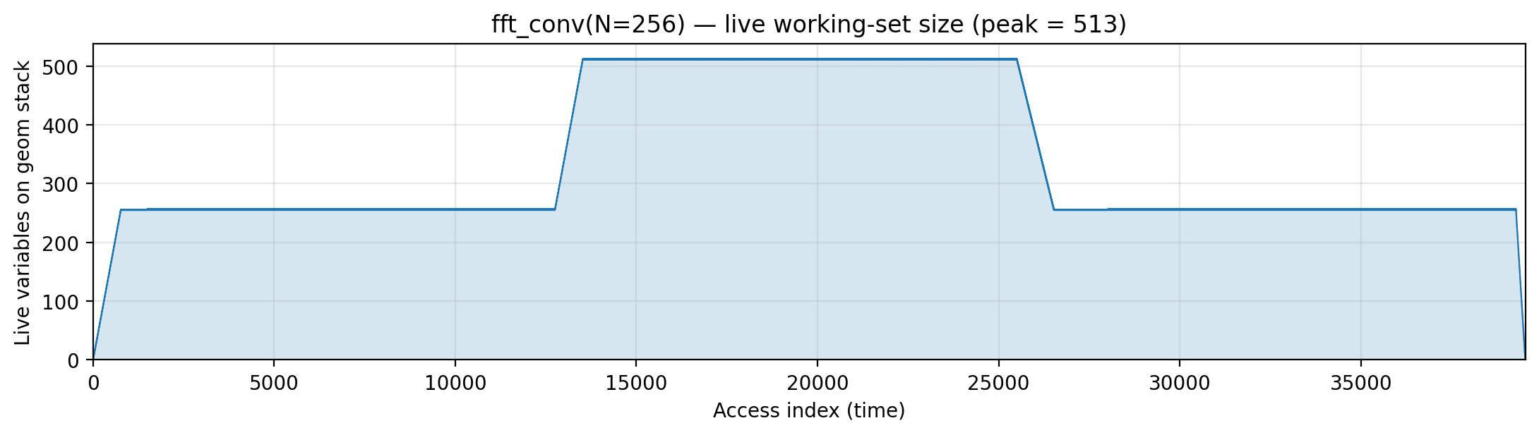
Working-set size over time (peak = 513).
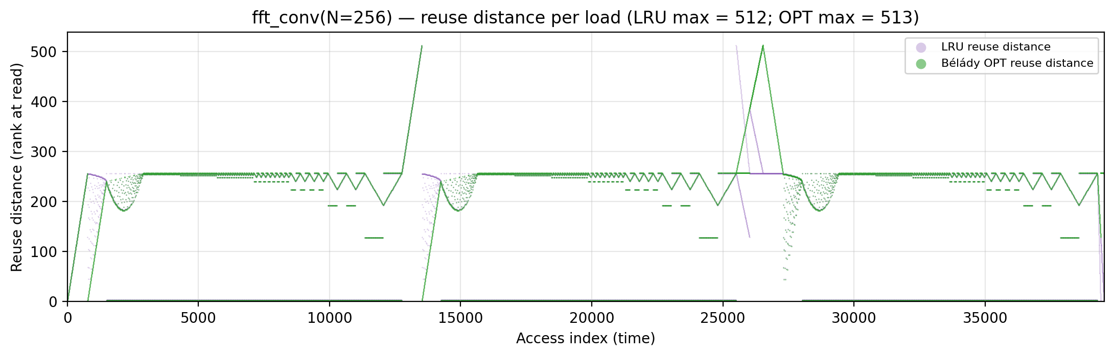
Reuse distance per load — LRU vs Bélády OPT (max LRU = 512; max OPT = 512).
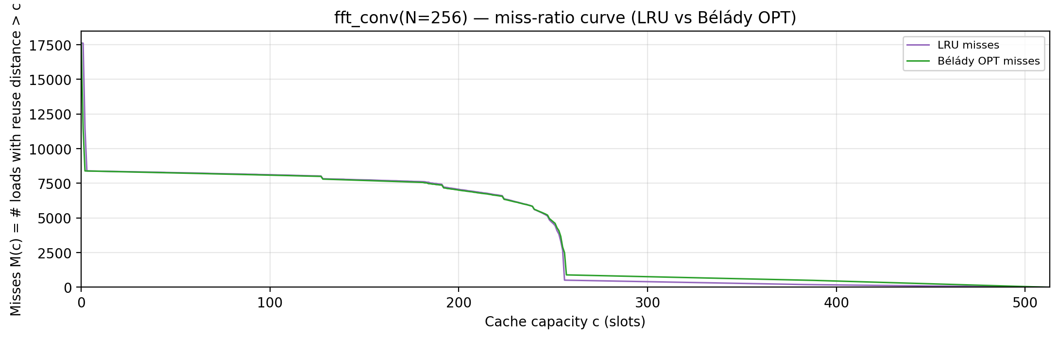
Miss-ratio curve — LRU vs Bélády OPT misses by cache capacity.
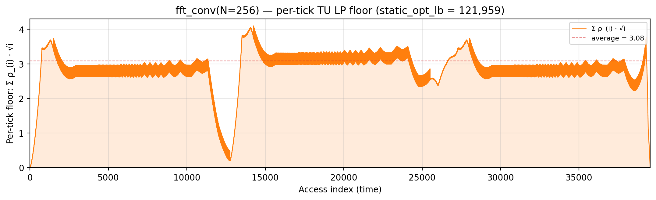
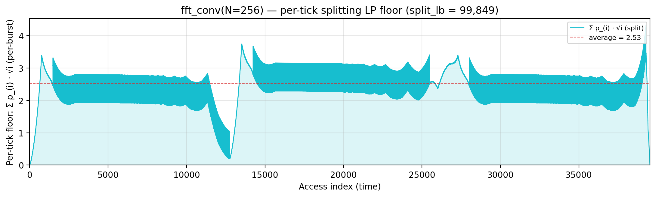
Per-tick TU LP floor — integrand of global_density: Σ_i ρ_{(i)} · √i over currently-live vars, ranked by density; the area equals global_density.
Per-tick splitting LP floor — integrand of local_density: Σ_i ρ_{(i)} · √i over the currently-active per-burst virtual intervals; the area equals the geometric portion of local_density.
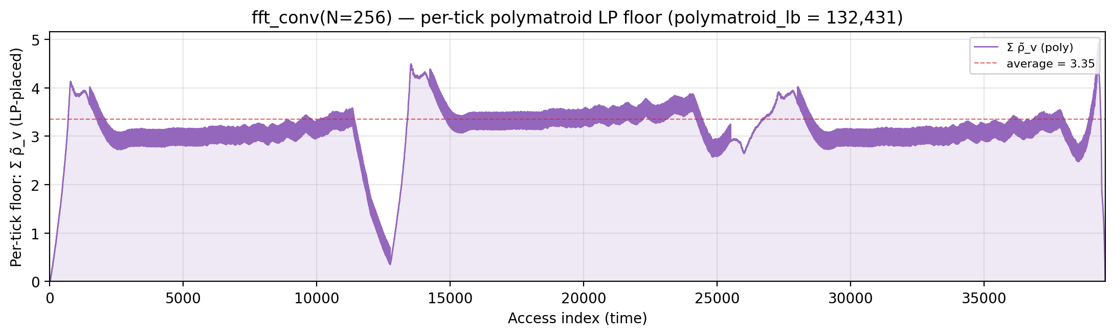
Per-tick polymatroid LP floor — integrand of polymatroid_lb: Σ_v reads_v · ⌈√d_v⌉ / lifespan(v) over live vars, where d_v is each variable’s LP-implied static depth (gemini/polymatroid-relaxation.md). The area equals the geometric portion of polymatroid_lb.
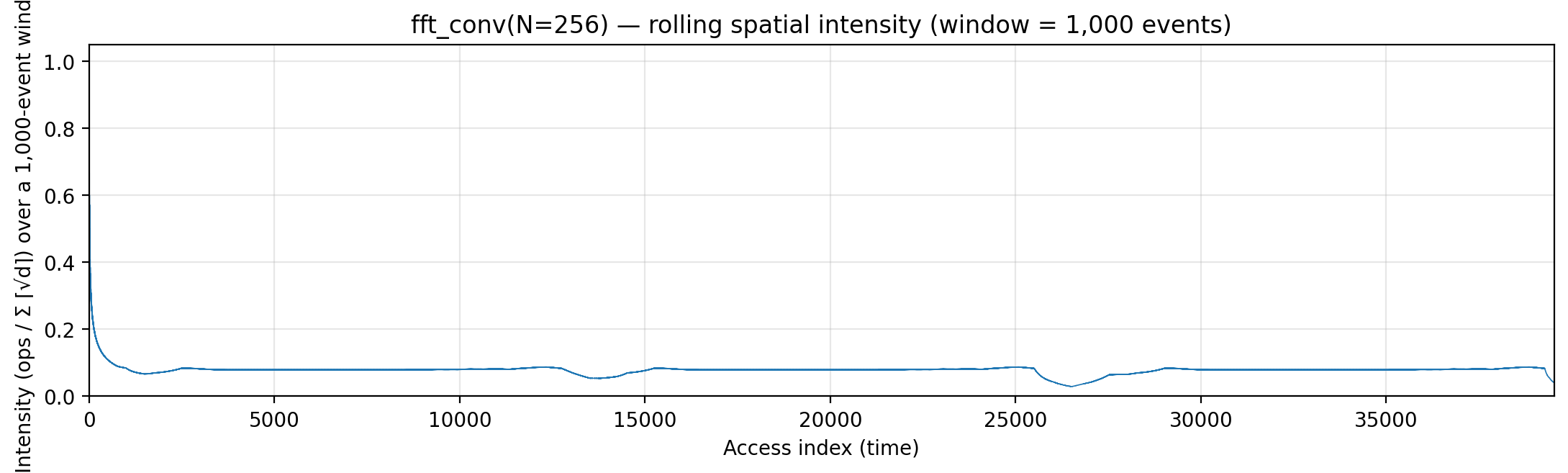
Rolling spatial intensity — heartbeat plot of ops / Σ ⌈√d⌉ over a sliding window.
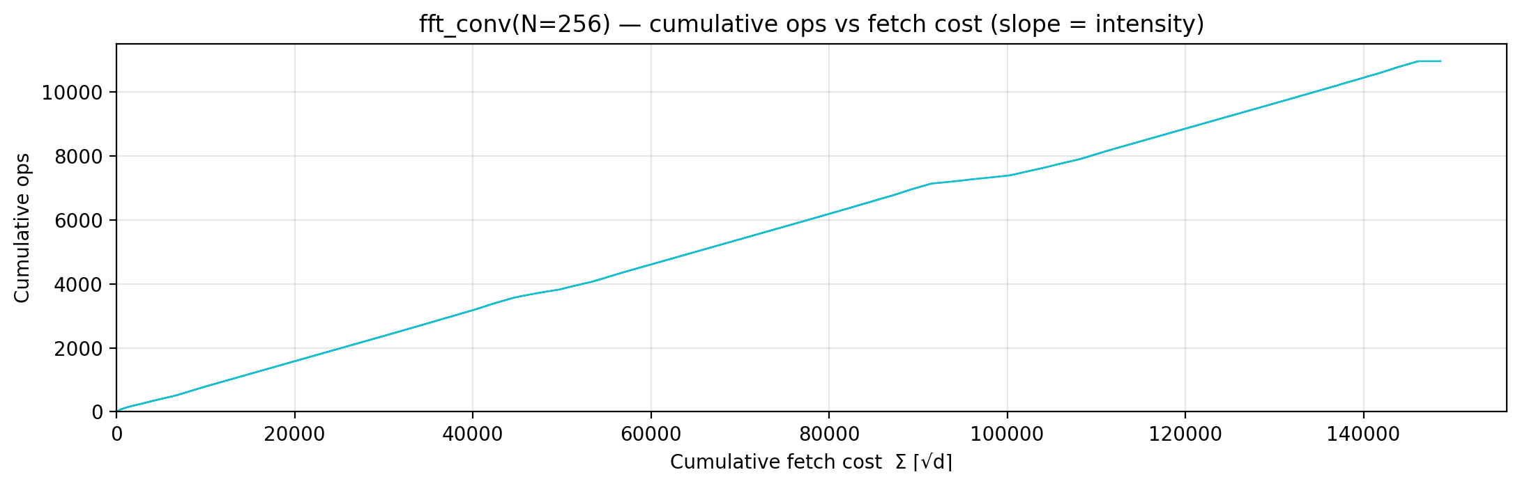
Cumulative compute vs fetch cost — slope = instantaneous spatial arithmetic intensity.
Gravity well — per-load fetch-cost ⌈√d⌉ scatter.
Spatial locality CDF — compute-fulfillment as a function of radius.
Working-set size over a τ = 100-event window (max = 100).
quicksort (code)
N=64. Algorithm. In-place recursive quicksort, data-oblivious
partition stand-in (_Tracked has no __lt__). At each level, scan
all sz-1 non-pivot elements, reading each with the pivot (2 reads,
result discarded). Recurses on two equal halves.
Manual placement. Only the input array at addrs 1..N — no temps,
since quicksort partitions in place. Pivot address is base + sz - 1
(highest slot in current subarray), which ends up at the “high”
address of each recursion window. manual (3,974) slightly exceeds
bytedmd_classic (3,661) because every pivot touch pays the full
⌈√(base+sz-1)⌉ under fixed placement, while LRU bumping would keep
the pivot at depth 1 after its first read inside the inner loop.
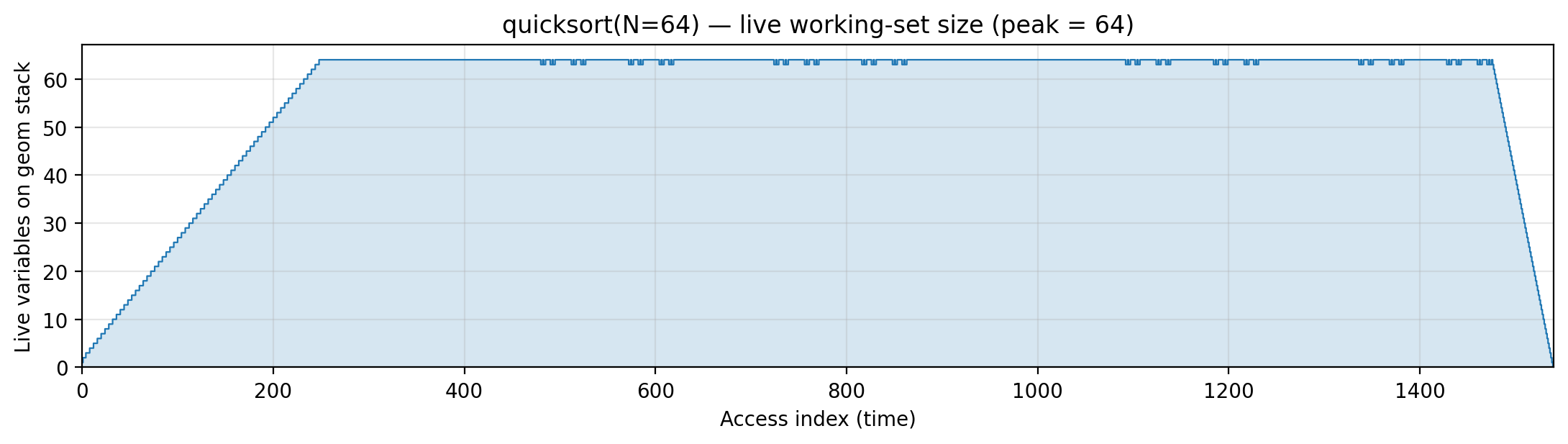
Working-set size over time (peak = 64).
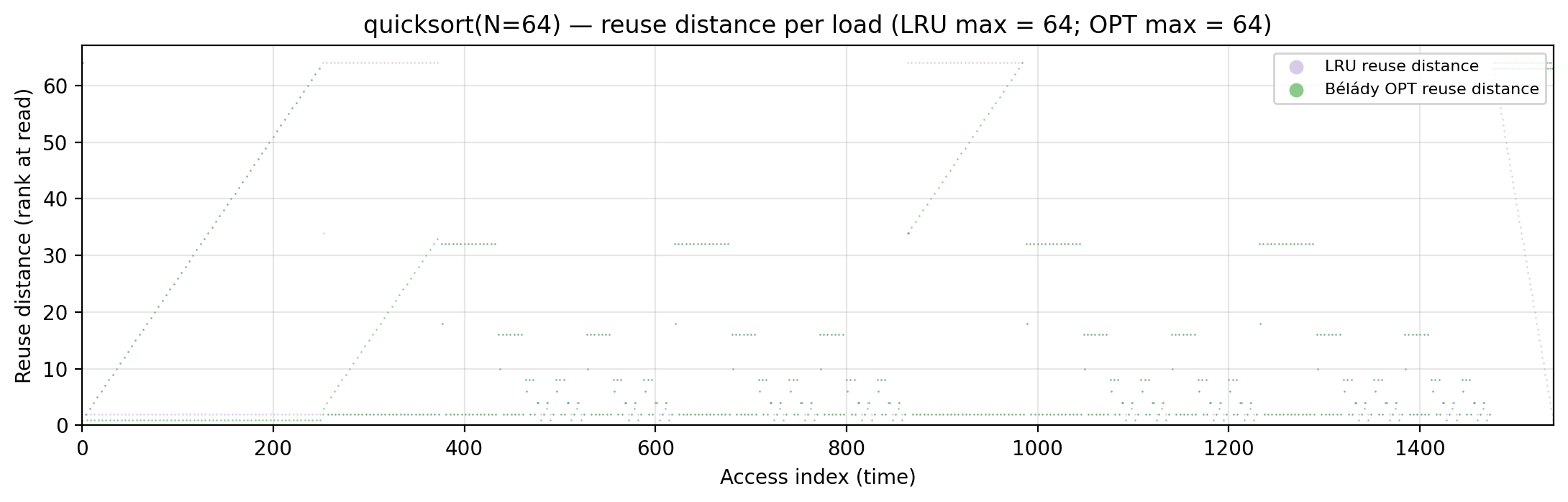
Reuse distance per load — LRU vs Bélády OPT (max LRU = 64; max OPT = 64).
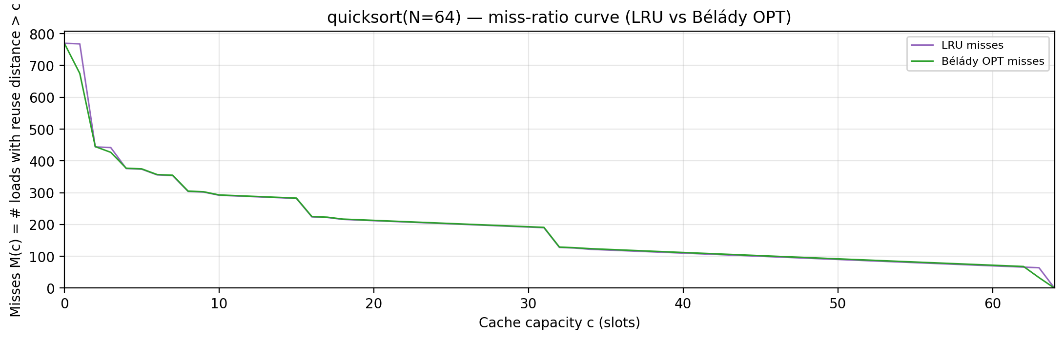
Miss-ratio curve — LRU vs Bélády OPT misses by cache capacity.
Per-tick TU LP floor — integrand of global_density: Σ_i ρ_{(i)} · √i over currently-live vars, ranked by density; the area equals global_density.

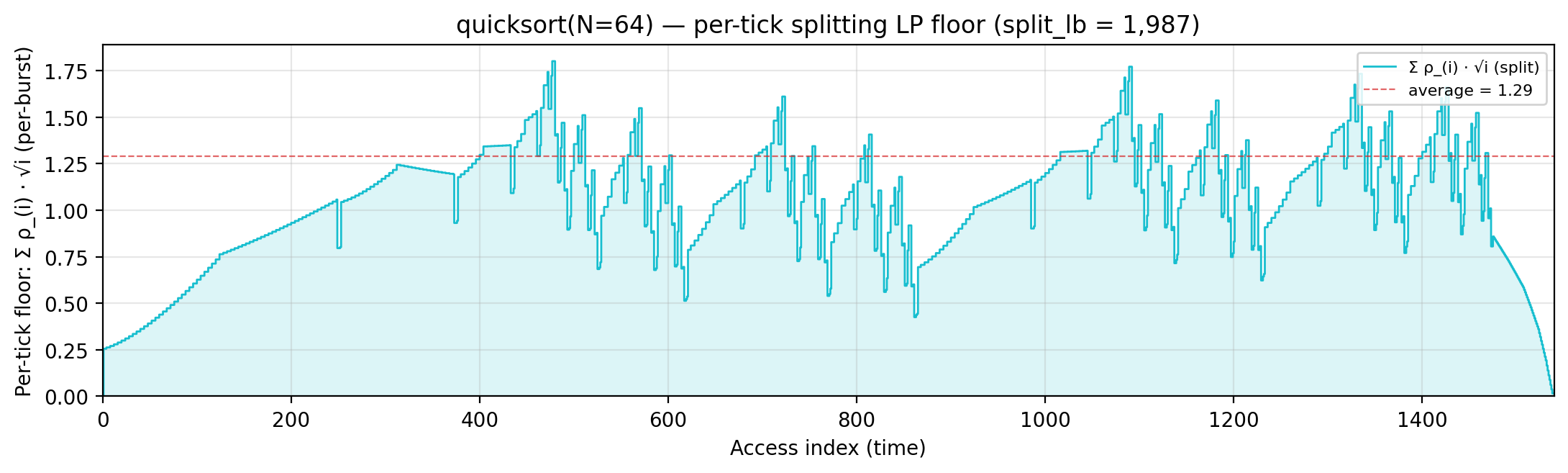
Per-tick splitting LP floor — integrand of local_density: Σ_i ρ_{(i)} · √i over the currently-active per-burst virtual intervals; the area equals the geometric portion of local_density.
Per-tick polymatroid LP floor — integrand of polymatroid_lb: Σ_v reads_v · ⌈√d_v⌉ / lifespan(v) over live vars, where d_v is each variable’s LP-implied static depth (gemini/polymatroid-relaxation.md). The area equals the geometric portion of polymatroid_lb.
Rolling spatial intensity — heartbeat plot of ops / Σ ⌈√d⌉ over a sliding window.
Cumulative compute vs fetch cost — slope = instantaneous spatial arithmetic intensity.
Gravity well — per-load fetch-cost ⌈√d⌉ scatter.
Spatial locality CDF — compute-fulfillment as a function of radius.
Working-set size over a τ = 57-event window (max = 57).
heapsort (code)
N=64. Algorithm. Two phases on an implicit binary max-heap:
build (sift-down from n/2-1 down to 0 to establish the heap
property) and extract (swap root with last, sift-down over
shrinking prefix, N-1 times). Each sift-down step reads parent and
one or two children at indices j, 2j+1, 2j+2, implementing the
classic tree-index address pattern.
Manual placement. In-place on the input array at addrs 1..N. The
heap’s tree structure means accesses always link a node at addr j
with its children at 2j+1 and 2j+2 — stride patterns that are
neither row-major nor column-major but follow the powers-of-2
backbone of a pointer-less heap. manual (4,779) lands between
bytedmd_live (4,548) and bytedmd_classic (7,164), and well under
mergesort’s 8,416 — in-place + no temps buys it a lot.
Working-set size over time (peak = 64).
Reuse distance per load — LRU vs Bélády OPT (max LRU = 64; max OPT = 64).
Miss-ratio curve — LRU vs Bélády OPT misses by cache capacity.
Per-tick TU LP floor — integrand of global_density: Σ_i ρ_{(i)} · √i over currently-live vars, ranked by density; the area equals global_density.
Per-tick splitting LP floor — integrand of local_density: Σ_i ρ_{(i)} · √i over the currently-active per-burst virtual intervals; the area equals the geometric portion of local_density.

Per-tick polymatroid LP floor — integrand of polymatroid_lb: Σ_v reads_v · ⌈√d_v⌉ / lifespan(v) over live vars, where d_v is each variable’s LP-implied static depth (gemini/polymatroid-relaxation.md). The area equals the geometric portion of polymatroid_lb.
Rolling spatial intensity — heartbeat plot of ops / Σ ⌈√d⌉ over a sliding window.
Cumulative compute vs fetch cost — slope = instantaneous spatial arithmetic intensity.
Gravity well — per-load fetch-cost ⌈√d⌉ scatter.
Spatial locality CDF — compute-fulfillment as a function of radius.
Working-set size over a τ = 36-event window (max = 36).
mergesort (code)
N=64. Algorithm. Recursive mergesort. Merge is implemented as a
data-oblivious stand-in (2 reads per output cell) since _Tracked
doesn’t implement __lt__ — the access traffic matches a real
comparison-based merge.
Manual placement. Perfect in-place oblivious merge with register
hoisting + an L1 scratchpad for the deep-subtree leaves (gemini’s
suggestion in gemini/optimize-mergesort.md):
c_A (addr 1) caches left[half-1] before the k-sweep;
c_B (addr 2) caches right[0] before the k-sweep;
S (addrs 3..10) is an 8-slot L1 scratchpad used for subtrees of
size ≤ 8 (leaves of the recursion tree);
arr (addrs 11..N+10) is the sole target array.
Because the oblivious merge pattern only repeats left[half-1] and
right[0] as clamped boundary reads, hoisting them into c_A/c_B
makes every in-place write of arr[base+k] safe — no temp buffers
at any level. Subtrees up to S_size compute in S; at the first
level where a half equals S_size we compute the left half in S,
copy to arr, then compute the right half in S and merge into arr.
Trajectory: 9,160 (original recursive push/pop) → 5,890 (my
ping-pong rewrite) → 3,386 (−63% from original). Now beats
bytedmd_classic (4,411) outright and is just 7.5% above
bytedmd_live (3,148).
Working-set size over time (peak = 65).
Reuse distance per load — LRU vs Bélády OPT (max LRU = 65; max OPT = 64).
Miss-ratio curve — LRU vs Bélády OPT misses by cache capacity.
Per-tick TU LP floor — integrand of global_density: Σ_i ρ_{(i)} · √i over currently-live vars, ranked by density; the area equals global_density.
Per-tick splitting LP floor — integrand of local_density: Σ_i ρ_{(i)} · √i over the currently-active per-burst virtual intervals; the area equals the geometric portion of local_density.
Per-tick polymatroid LP floor — integrand of polymatroid_lb: Σ_v reads_v · ⌈√d_v⌉ / lifespan(v) over live vars, where d_v is each variable’s LP-implied static depth (gemini/polymatroid-relaxation.md). The area equals the geometric portion of polymatroid_lb.
Rolling spatial intensity — heartbeat plot of ops / Σ ⌈√d⌉ over a sliding window.
Cumulative compute vs fetch cost — slope = instantaneous spatial arithmetic intensity.
Gravity well — per-load fetch-cost ⌈√d⌉ scatter.
Spatial locality CDF — compute-fulfillment as a function of radius.
Working-set size over a τ = 51-event window (max = 51).
lcs_dp (code)
m=n=32. Algorithm. Longest-common-subsequence dynamic programming
on an (m+1)×(n+1) table, row-major fill. Branch-free sum replaces the
max/equality recurrence; access pattern matches canonical LCS:
3 table reads + 2 string reads per cell.
Manual placement. Since the algorithm only returns D[m][n], the
full (m+1)(n+1) table is unnecessary — use a rolling 2-row buffer
with a pivot scalar at the bottom of the stack:
c_A (addr 1) holds x[i-1] as the hot pivot for the j-sweep;
row_a, row_b (addrs 2..2n+3) ping-pong as previous/current rows.
All three DP neighbour reads hit these low-address buffers. Drops
manual from 80,940 to 27,192 (−66%), just above global_density
(20,494) and roughly tied with bytedmd_live (25,572).
Working-set size over time (peak = 97).
Reuse distance per load — LRU vs Bélády OPT (max LRU = 96; max OPT = 65).
Miss-ratio curve — LRU vs Bélády OPT misses by cache capacity.
Per-tick TU LP floor — integrand of global_density: Σ_i ρ_{(i)} · √i over currently-live vars, ranked by density; the area equals global_density.
Per-tick splitting LP floor — integrand of local_density: Σ_i ρ_{(i)} · √i over the currently-active per-burst virtual intervals; the area equals the geometric portion of local_density.
Per-tick polymatroid LP floor — integrand of polymatroid_lb: Σ_v reads_v · ⌈√d_v⌉ / lifespan(v) over live vars, where d_v is each variable’s LP-implied static depth (gemini/polymatroid-relaxation.md). The area equals the geometric portion of polymatroid_lb.
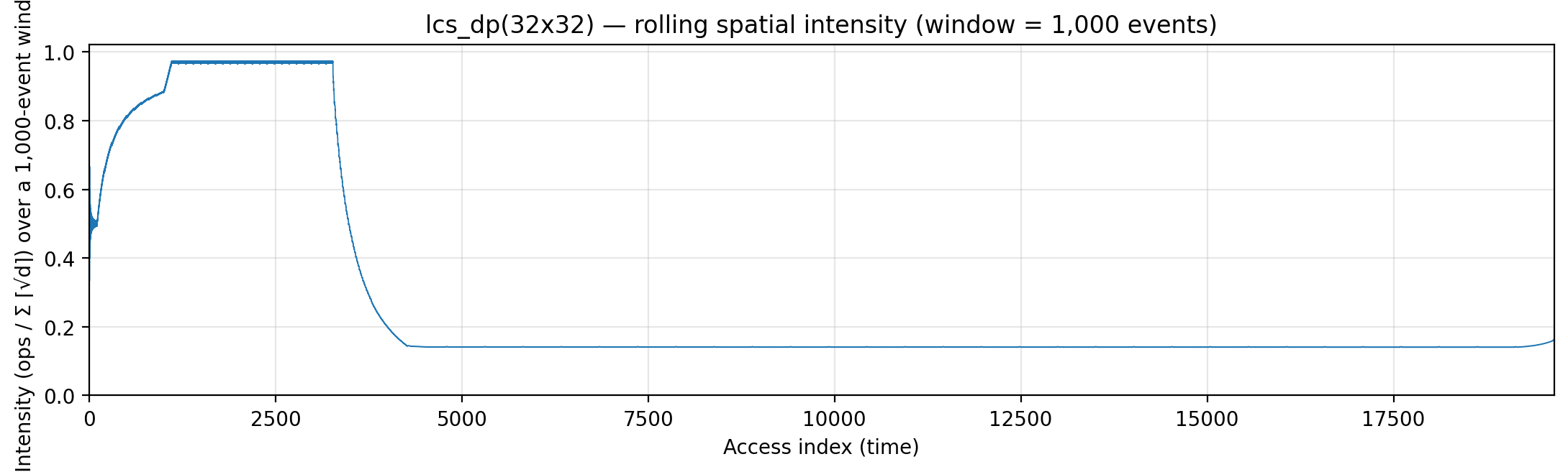
Rolling spatial intensity — heartbeat plot of ops / Σ ⌈√d⌉ over a sliding window.
Cumulative compute vs fetch cost — slope = instantaneous spatial arithmetic intensity.
Gravity well — per-load fetch-cost ⌈√d⌉ scatter.
Spatial locality CDF — compute-fulfillment as a function of radius.
Working-set size over a τ = 66-event window (max = 31).
lu_no_pivot (code)
n=32. Algorithm. Doolittle-style Gaussian elimination without
pivoting. For each k: read pivot A[k][k], scale subdiagonal
column A[k+1:,k], then rank-1 update the trailing submatrix
A[k+1:, k+1:] -= A[k+1:, k] · A[k, k+1:]. Classical O(n³/3)
triple loop.
Manual placement. Two hoisted scratchpads at the bottom of the
stack replace the bulk-only schedule:
c_A (addr 1) pins the pivot and then A[i][k] during the Schur
rank-1 update;
c_C (addrs 2..n+1) caches row k’s trailing tail A[k][k+1..].
Combined with lazy arg-stack reads (no upfront n² preload — each A
cell is touched from the arg stack on its first visit at k=0), the
Schur inner loop reads exactly one bulk A cell (the destination)
plus two hot scratchpad cells. Drops manual from 751,252 to
382,440 (−49%), now within 2 % of bytedmd_live (393,809).
Working-set size over time (peak = 1,025).
Reuse distance per load — LRU vs Bélády OPT (max LRU = 1,024; max OPT = 1,024).
Miss-ratio curve — LRU vs Bélády OPT misses by cache capacity.
Per-tick TU LP floor — integrand of global_density: Σ_i ρ_{(i)} · √i over currently-live vars, ranked by density; the area equals global_density.

Per-tick splitting LP floor — integrand of local_density: Σ_i ρ_{(i)} · √i over the currently-active per-burst virtual intervals; the area equals the geometric portion of local_density.

Rolling spatial intensity — heartbeat plot of ops / Σ ⌈√d⌉ over a sliding window.
Cumulative compute vs fetch cost — slope = instantaneous spatial arithmetic intensity.
Gravity well — per-load fetch-cost ⌈√d⌉ scatter.
Spatial locality CDF — compute-fulfillment as a function of radius.
Working-set size over a τ = 763-event window (max = 763).
blocked_lu (code)
n=32, NB=8. Algorithm. Block LU with four-step pattern per
diagonal block: (a) factor the NB×NB block via naive LU; (b)
triangular-solve the trailing column panel; (c) triangular-solve the
trailing row strip; (d) GEMM-update the trailing submatrix.
Manual placement. Three tight scratchpads at the very bottom of
the stack (addrs 1..73): a scalar c_A, a 1D row buffer c_C[NB],
and a 2D block buffer c_B[NB×NB]. c_B is multiplexed across all
four stages (diagonal factor, panel update, row-strip update,
trailing GEMM); c_C caches the currently-active A-row during the
panel and GEMM inner loops so every (i, j, k) triple-loop body
reads from addresses 1..73 only. The n² up-front preload is also
skipped — each A cell is touched lazily from the arg stack on its
first visit (when kb == 0) and from scratch A thereafter
(gemini/optimize-blocked-lu.md).
These three changes together drop the manual cost 870,705 →
236,290 (–73 %), now below bytedmd_live (283,294) — the manual
schedule wins because it can actively hoist hot operands that the
dynamic LRU heuristic can only approximate.
Working-set size over time (peak = 1,025).
Reuse distance per load — LRU vs Bélády OPT (max LRU = 1,024; max OPT = 1,024).
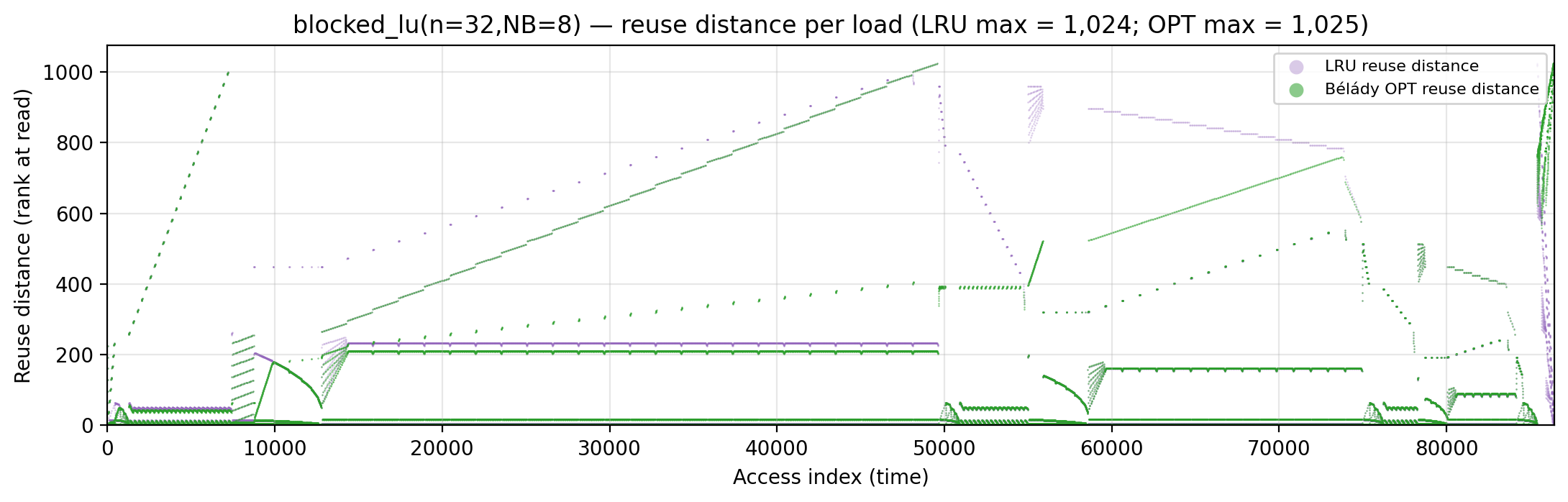
Miss-ratio curve — LRU vs Bélády OPT misses by cache capacity.
Per-tick TU LP floor — integrand of global_density: Σ_i ρ_{(i)} · √i over currently-live vars, ranked by density; the area equals global_density.
Per-tick splitting LP floor — integrand of local_density: Σ_i ρ_{(i)} · √i over the currently-active per-burst virtual intervals; the area equals the geometric portion of local_density.
Rolling spatial intensity — heartbeat plot of ops / Σ ⌈√d⌉ over a sliding window.
Cumulative compute vs fetch cost — slope = instantaneous spatial arithmetic intensity.
Gravity well — per-load fetch-cost ⌈√d⌉ scatter.
Spatial locality CDF — compute-fulfillment as a function of radius.
Working-set size over a τ = 233-event window (max = 233).
recursive_lu (code)
n=32. Algorithm. Cache-oblivious divide-and-conquer: split A
into 2×2 quadrants, factor A11 recursively, triangular-solve A12/A21,
Schur-complement A22, recurse on A22. Equivalent FLOP count to the
triple-loop version but with a block-decomposed access pattern.
Manual placement. Three hoisted scratchpads cover all three
Schur-style inner loops:
c_A (addr 1) pivot scalar,
c_B (addr 2) column-k scalar (A[i][k]),
c_C (addrs 3..n+2) row-k trailing buffer.
Each inner A[i][j] -= A[i][k] * A[k][j] body now reads one bulk
cell and two hot scratchpads instead of three bulk reads (lazy
loading is skipped because “first touch” under the recursion is
hard to define statically, so we keep the upfront preload). Drops
manual from 750,560 to 440,803 (−41%) — recursive_lu still
edges above global_density (238,782) because some of the lower-panel
traffic can’t be amortized into the scratchpads across recursion
levels.
Working-set size over time (peak = 1,025).
Reuse distance per load — LRU vs Bélády OPT (max LRU = 1,024; max OPT = 1,024).
Miss-ratio curve — LRU vs Bélády OPT misses by cache capacity.
Per-tick TU LP floor — integrand of global_density: Σ_i ρ_{(i)} · √i over currently-live vars, ranked by density; the area equals global_density.
Per-tick splitting LP floor — integrand of local_density: Σ_i ρ_{(i)} · √i over the currently-active per-burst virtual intervals; the area equals the geometric portion of local_density.
Rolling spatial intensity — heartbeat plot of ops / Σ ⌈√d⌉ over a sliding window.
Cumulative compute vs fetch cost — slope = instantaneous spatial arithmetic intensity.
Gravity well — per-load fetch-cost ⌈√d⌉ scatter.
Spatial locality CDF — compute-fulfillment as a function of radius.
Working-set size over a τ = 305-event window (max = 305).
lu_partial_pivot (code)
n=32. Algorithm. Same elimination as lu_no_pivot but each
step first scans column k for the max-magnitude pivot and swaps that
row into position. Data-oblivious stand-in: pretend the pivot is
always row k+1 and perform the swap unconditionally.
Manual placement. Same hoisted scratchpads as lu_no_pivot
(c_A + c_C) plus lazy arg-stack reads. The column scan and
row swap run before the scratchpads are primed, so they pay bulk-A
cost; the expensive part (Schur rank-1 update) uses the hot
scratchpads the same way. Drops manual from 793,416 to 427,384
(−46%); the LP lower bound is 263,705, which the manual schedule
still overshoots by ≈62 % because the in-place trace can’t be
fully exploited from a static layout.
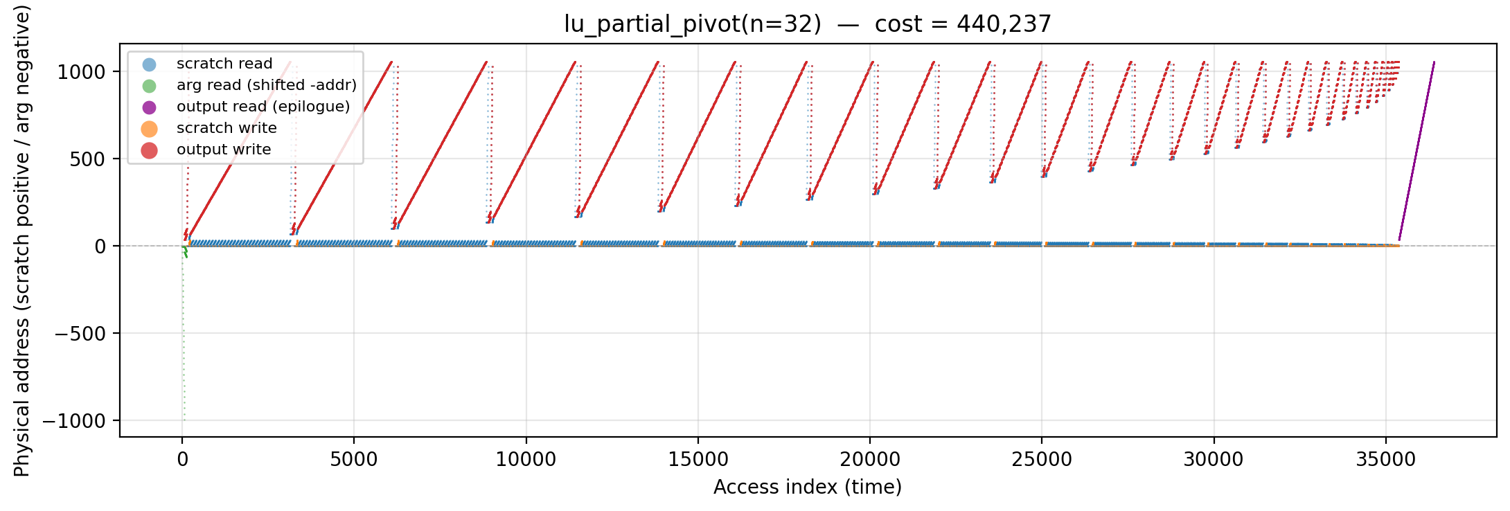
Working-set size over time (peak = 1,025).
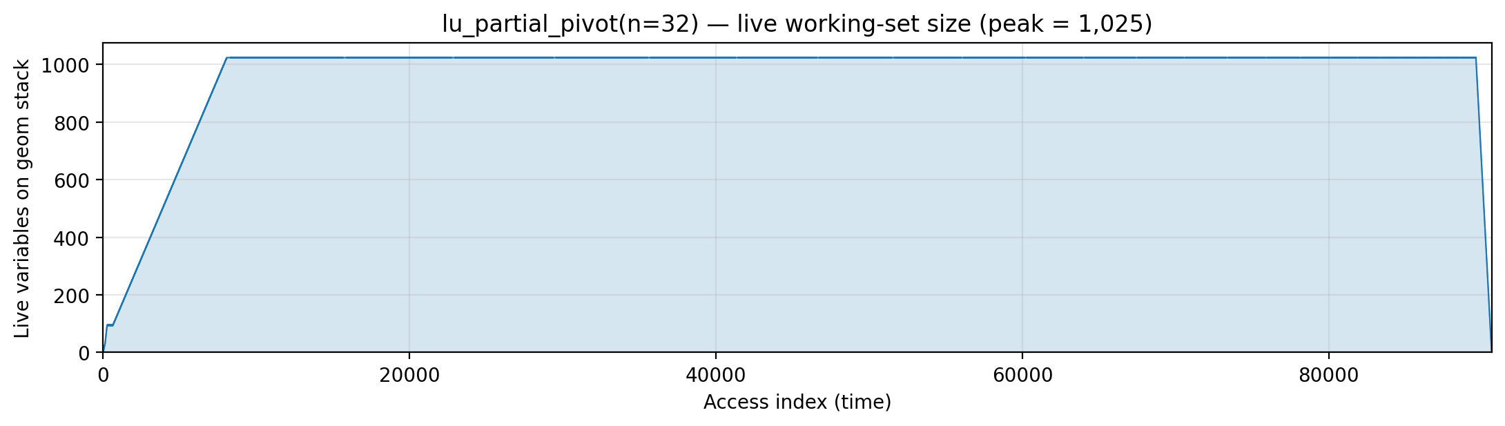
Reuse distance per load — LRU vs Bélády OPT (max LRU = 1,024; max OPT = 1,024).
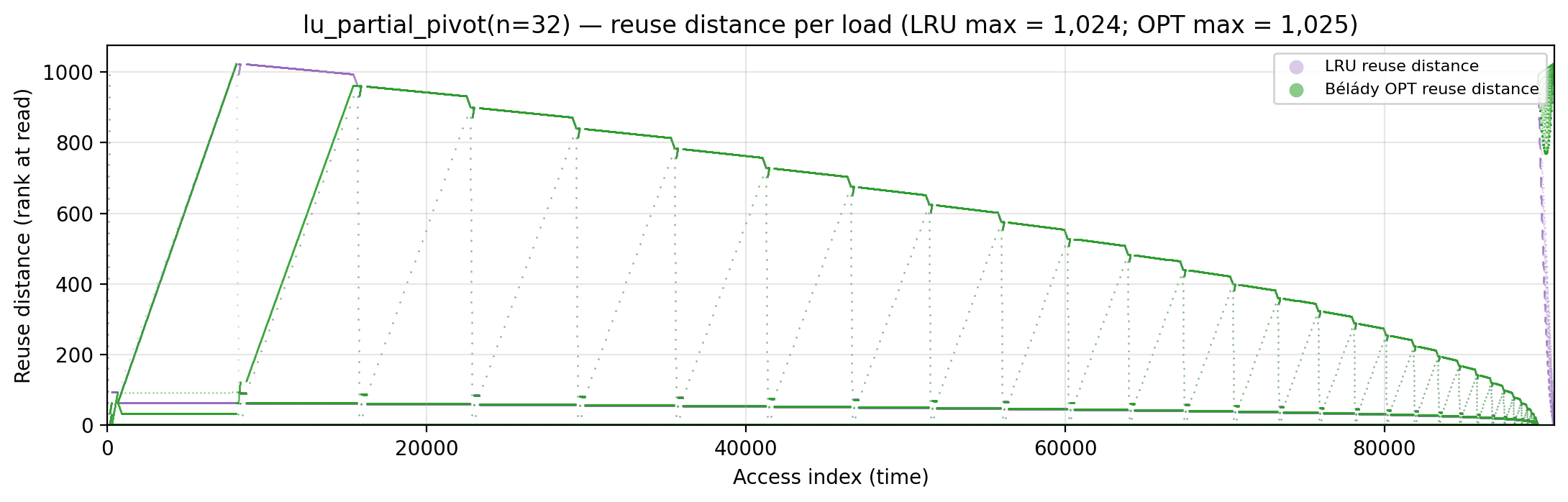
Miss-ratio curve — LRU vs Bélády OPT misses by cache capacity.
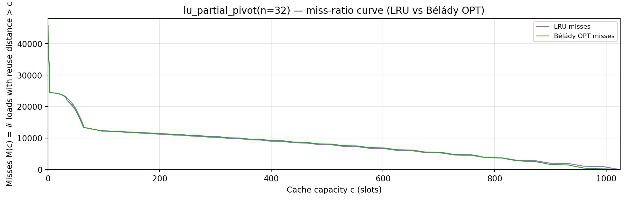
Per-tick TU LP floor — integrand of global_density: Σ_i ρ_{(i)} · √i over currently-live vars, ranked by density; the area equals global_density.
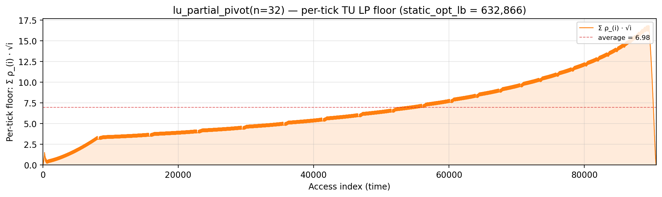
Per-tick splitting LP floor — integrand of local_density: Σ_i ρ_{(i)} · √i over the currently-active per-burst virtual intervals; the area equals the geometric portion of local_density.
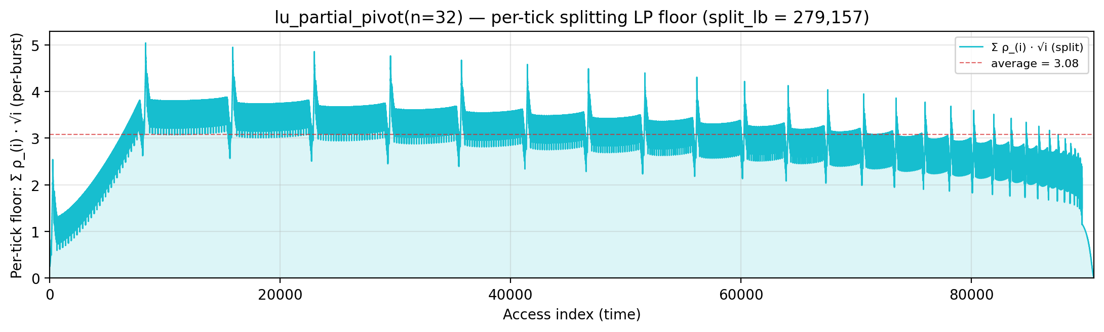
Rolling spatial intensity — heartbeat plot of ops / Σ ⌈√d⌉ over a sliding window.
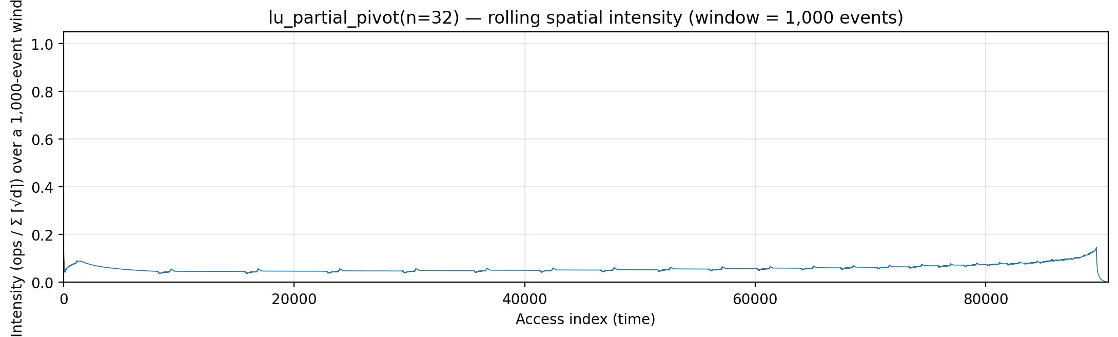
Cumulative compute vs fetch cost — slope = instantaneous spatial arithmetic intensity.
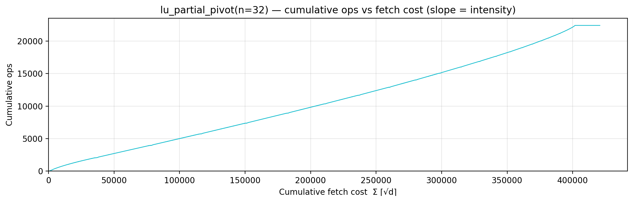
Gravity well — per-load fetch-cost ⌈√d⌉ scatter.
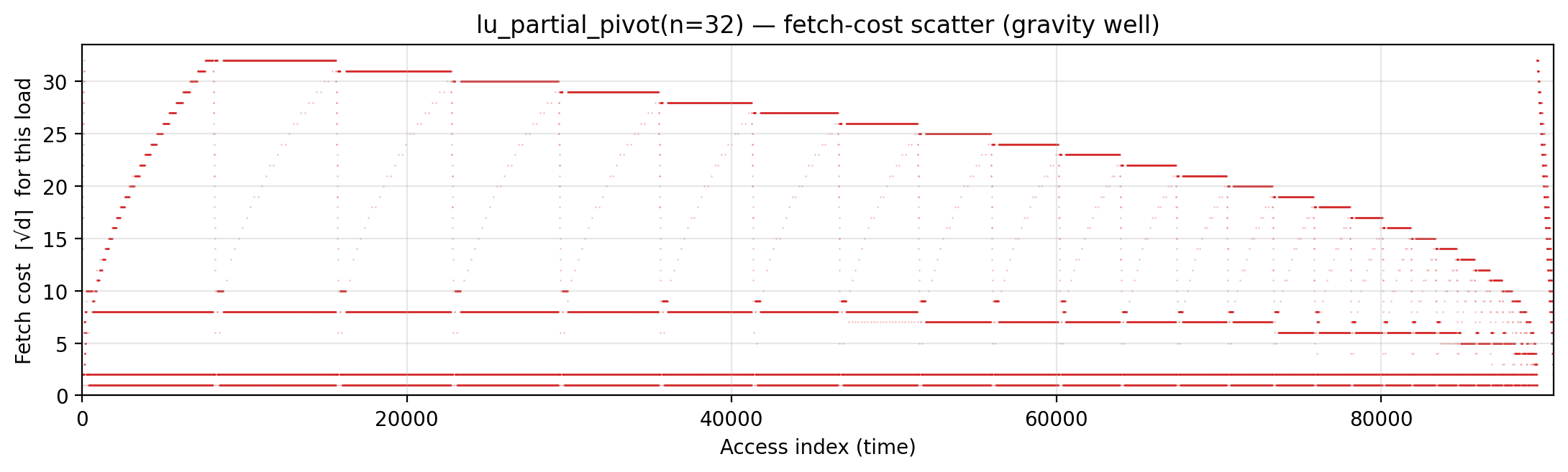
Spatial locality CDF — compute-fulfillment as a function of radius.
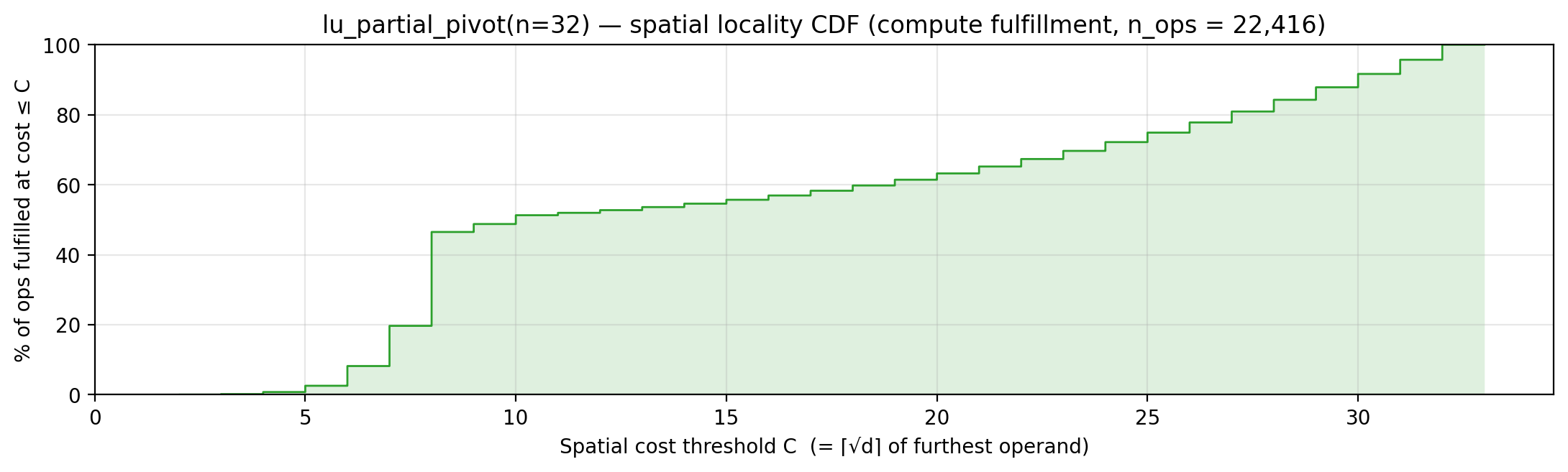
Working-set size over a τ = 735-event window (max = 735).
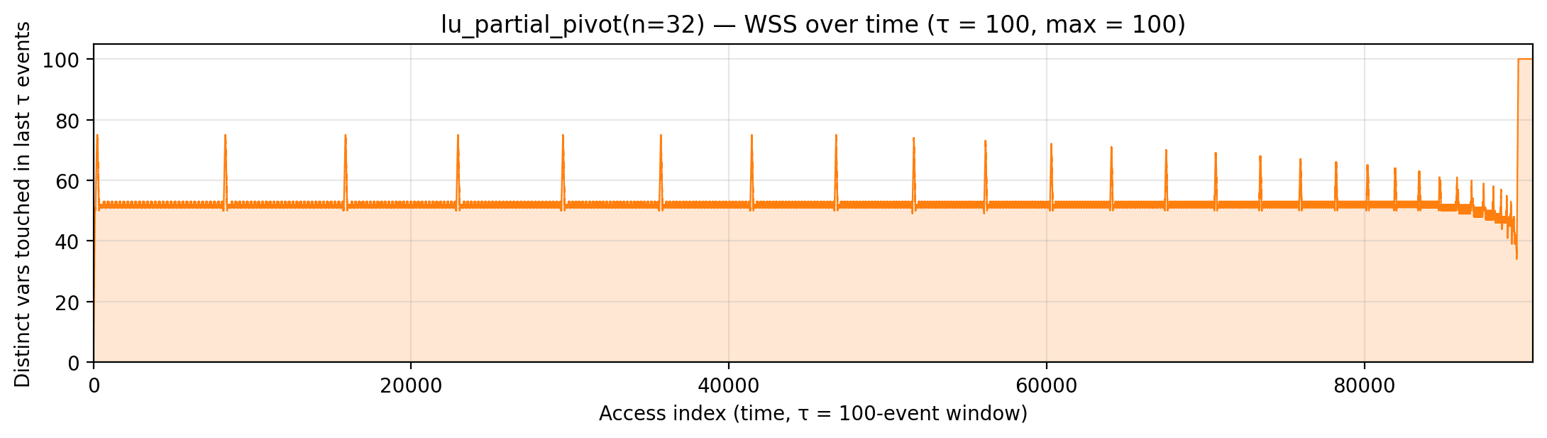
cholesky (code)
n=32. Algorithm. Right-looking Cholesky for an SPD matrix:
factor A = L·Lᵀ in place, reading only the lower triangle. For
each k: stand-in-sqrt on A[k][k], scale A[k+1:, k], rank-1
update A[i][j] -= A[i][k]·A[j][k] for i ≥ j > k.
Manual placement. c_A (addr 1) pins the pivot then A[j][k]
during the Schur inner i-sweep; c_C (addrs 2..n+1) caches column
k below the diagonal for the full Schur update. Lazy arg-stack
reads replace the n² preload. Inner A[i][j] -= A[i][k] * A[j][k]
body reads one bulk cell plus two hot scratchpads. Drops manual
from 494,000 to 238,688 (−52%), still above global_density
(124,333) but well below bytedmd_classic (293,328).
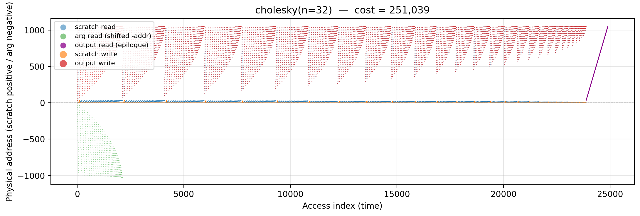
Working-set size over time (peak = 529).
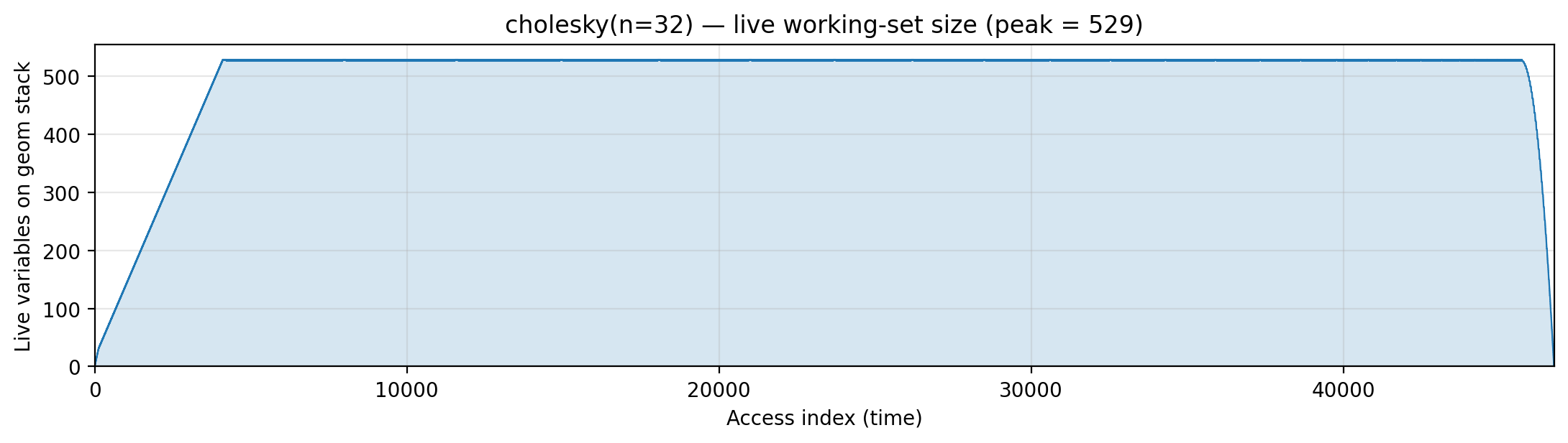
Reuse distance per load — LRU vs Bélády OPT (max LRU = 1,024; max OPT = 1,024).
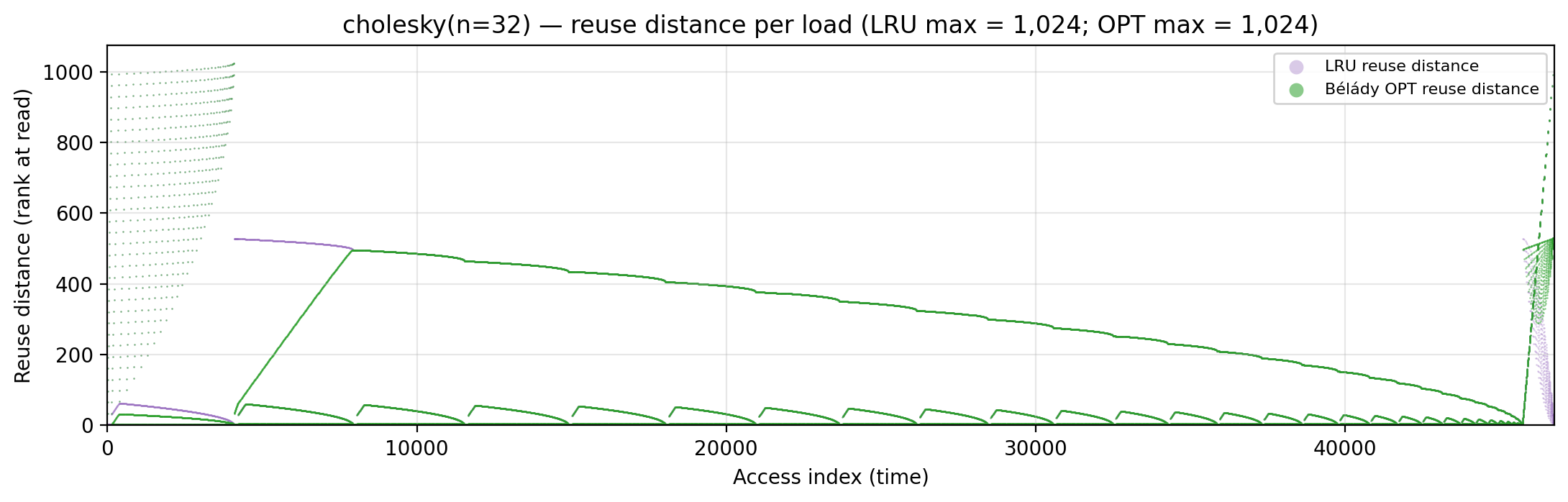
Miss-ratio curve — LRU vs Bélády OPT misses by cache capacity.
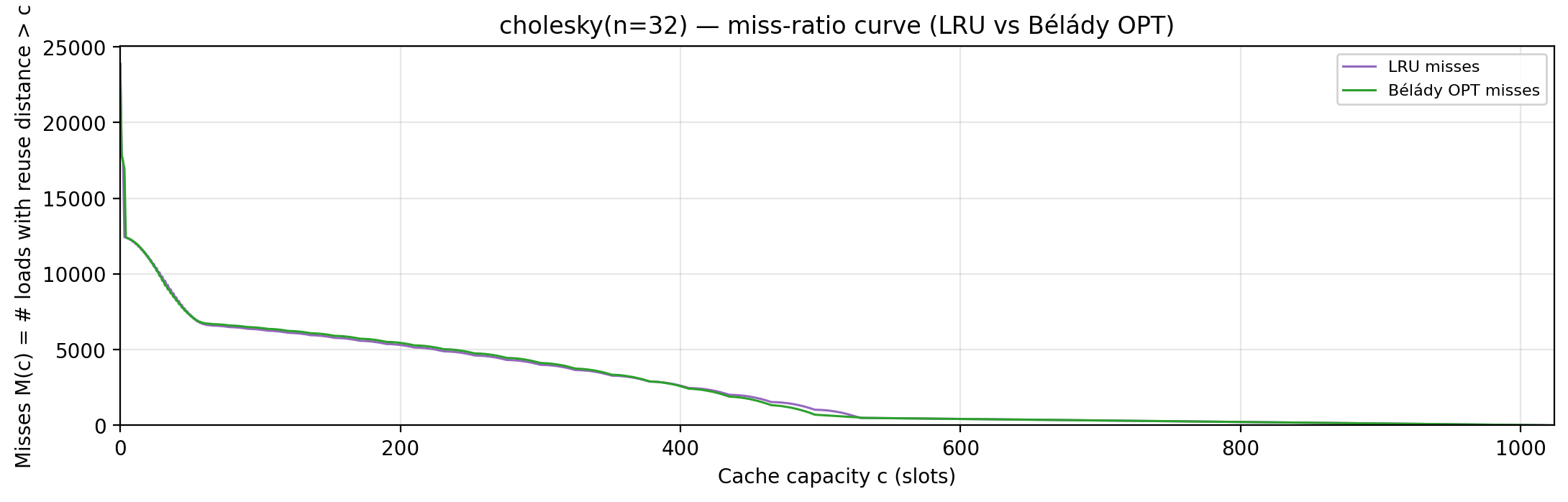
Per-tick TU LP floor — integrand of global_density: Σ_i ρ_{(i)} · √i over currently-live vars, ranked by density; the area equals global_density.
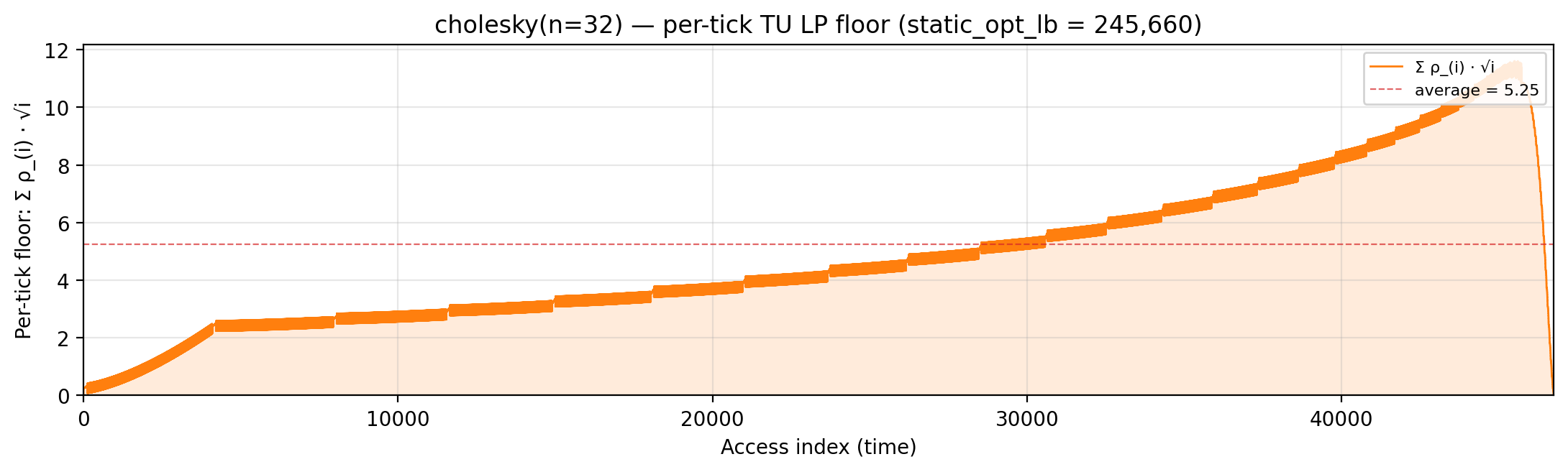
Per-tick splitting LP floor — integrand of local_density: Σ_i ρ_{(i)} · √i over the currently-active per-burst virtual intervals; the area equals the geometric portion of local_density.
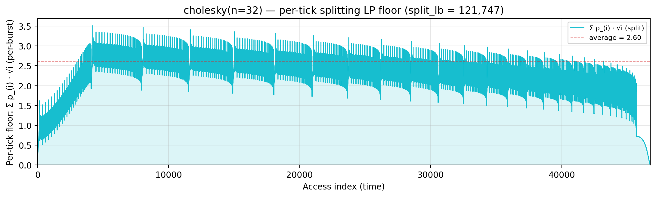
Rolling spatial intensity — heartbeat plot of ops / Σ ⌈√d⌉ over a sliding window.
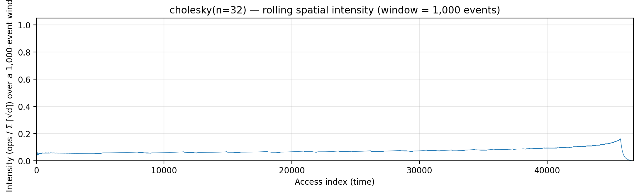
Cumulative compute vs fetch cost — slope = instantaneous spatial arithmetic intensity.
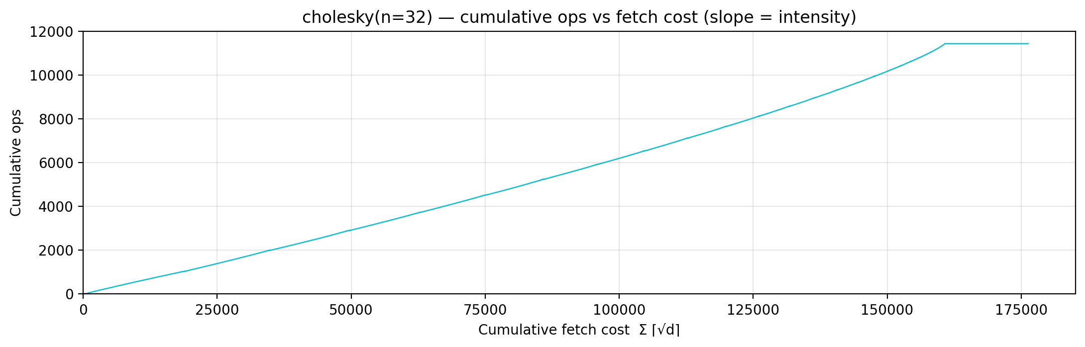
Gravity well — per-load fetch-cost ⌈√d⌉ scatter.
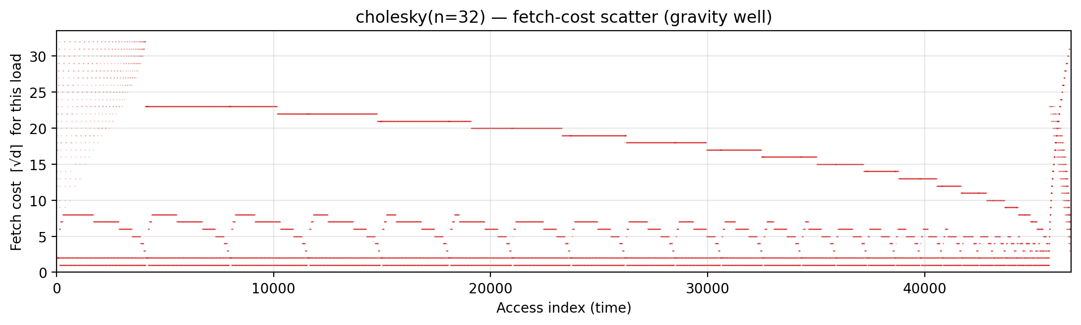
Spatial locality CDF — compute-fulfillment as a function of radius.
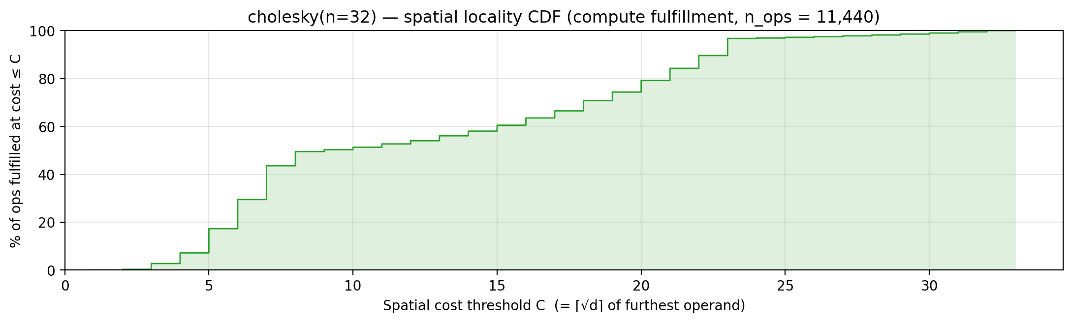
Working-set size over a τ = 418-event window (max = 418).
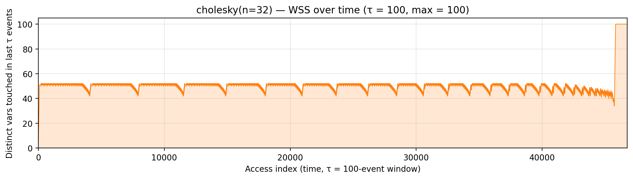
householder_qr (code)
32×32. Algorithm. Classical Householder QR: for each column k,
compute a reflector from A[k:m, k], apply it to each trailing
column A[k:m, k+1:n] (dot-product then rank-1 update). Access
pattern matches LAPACK’s DGEQR2.
Manual placement. Two hoisted scratchpads at the bottom of the
stack turn the “apply reflector” phase into 1 bulk read + 2 hot reads
per inner op:
c_A (addr 1) accumulates the dot product;
c_V (addrs 2..m+1) caches the reflector column once per k and is
re-read across all n trailing columns j.
Drops manual from 1,146,072 to 743,882 (−35%), now within 21 %
of bytedmd_live (615,355).
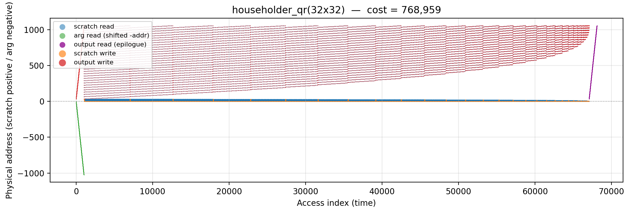
Working-set size over time (peak = 1,026).
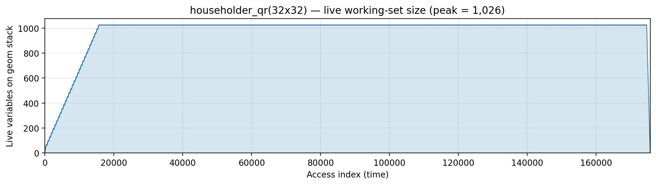
Reuse distance per load — LRU vs Bélády OPT (max LRU = 1,024; max OPT = 1,024).
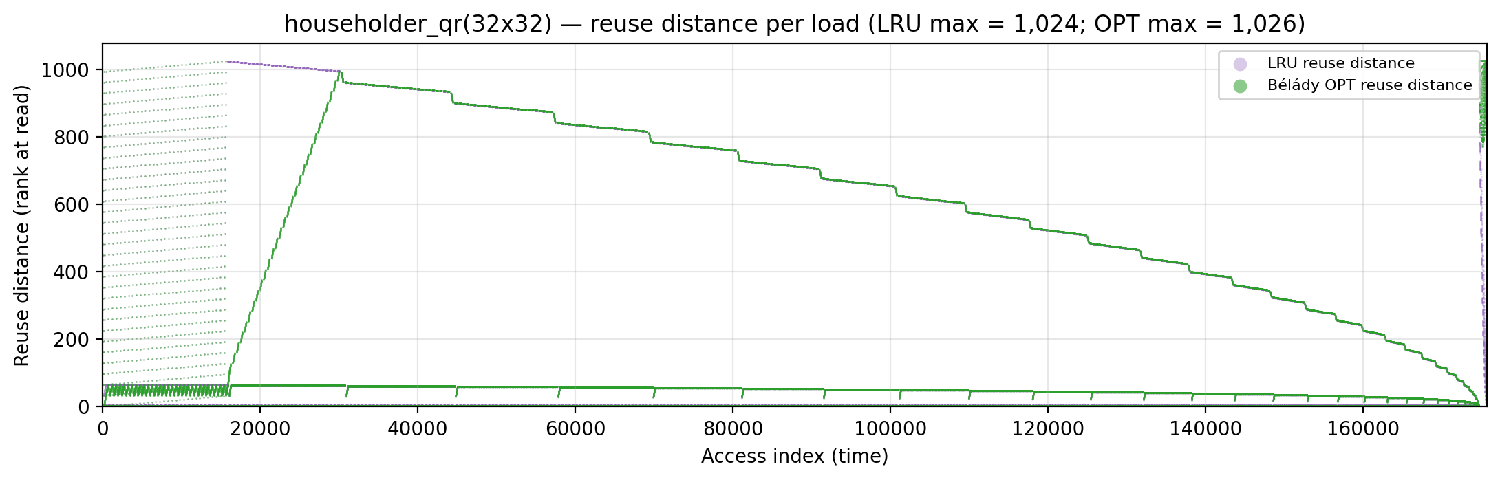
Miss-ratio curve — LRU vs Bélády OPT misses by cache capacity.
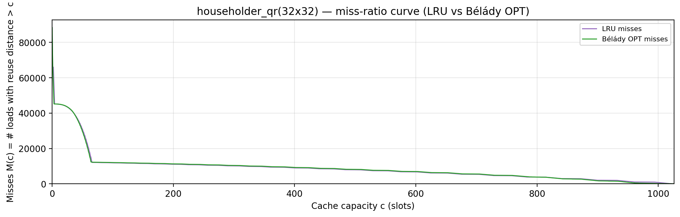
Per-tick TU LP floor — integrand of global_density: Σ_i ρ_{(i)} · √i over currently-live vars, ranked by density; the area equals global_density.
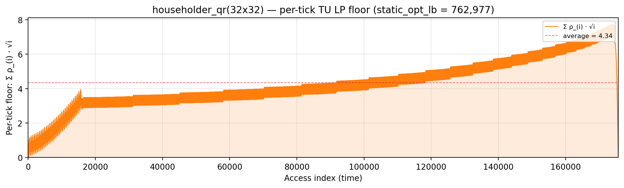
Per-tick splitting LP floor — integrand of local_density: Σ_i ρ_{(i)} · √i over the currently-active per-burst virtual intervals; the area equals the geometric portion of local_density.
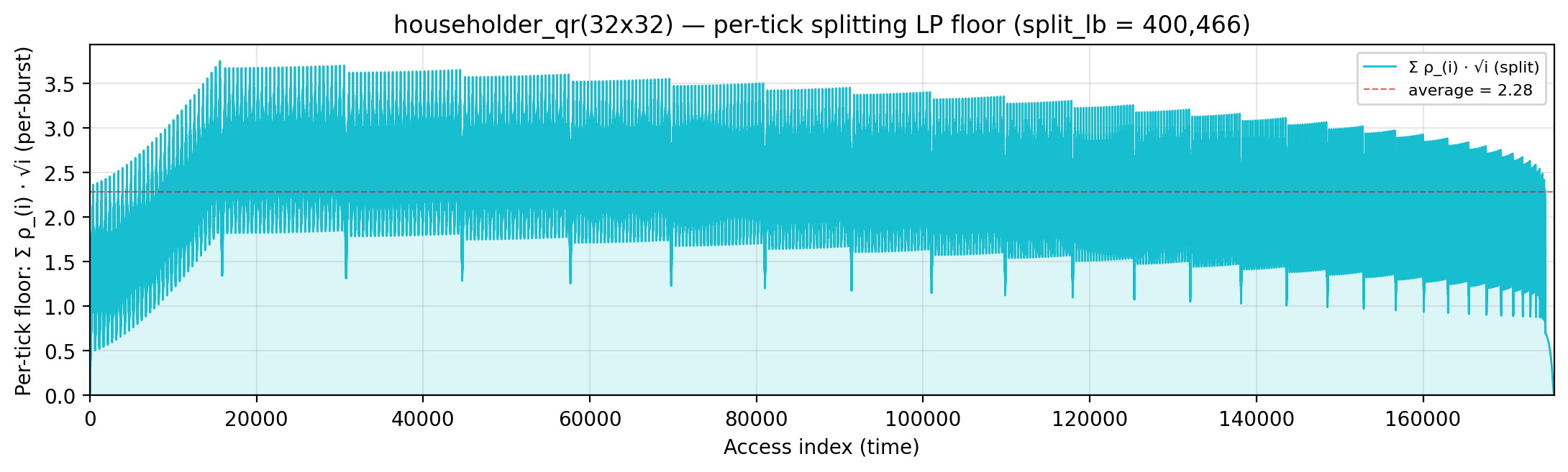
Rolling spatial intensity — heartbeat plot of ops / Σ ⌈√d⌉ over a sliding window.
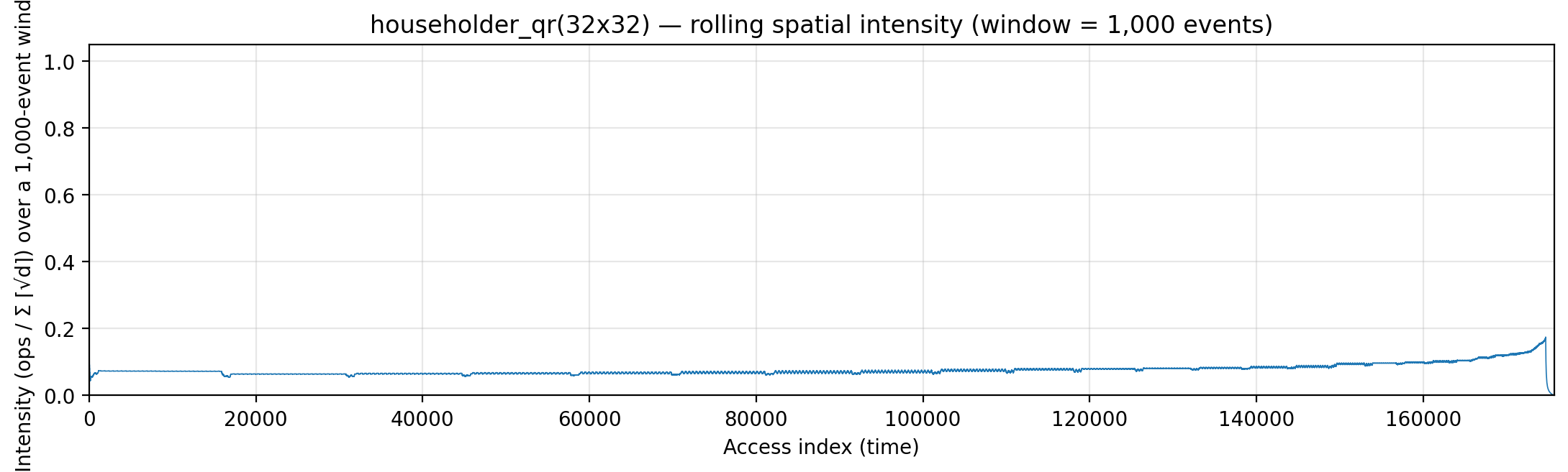
Cumulative compute vs fetch cost — slope = instantaneous spatial arithmetic intensity.
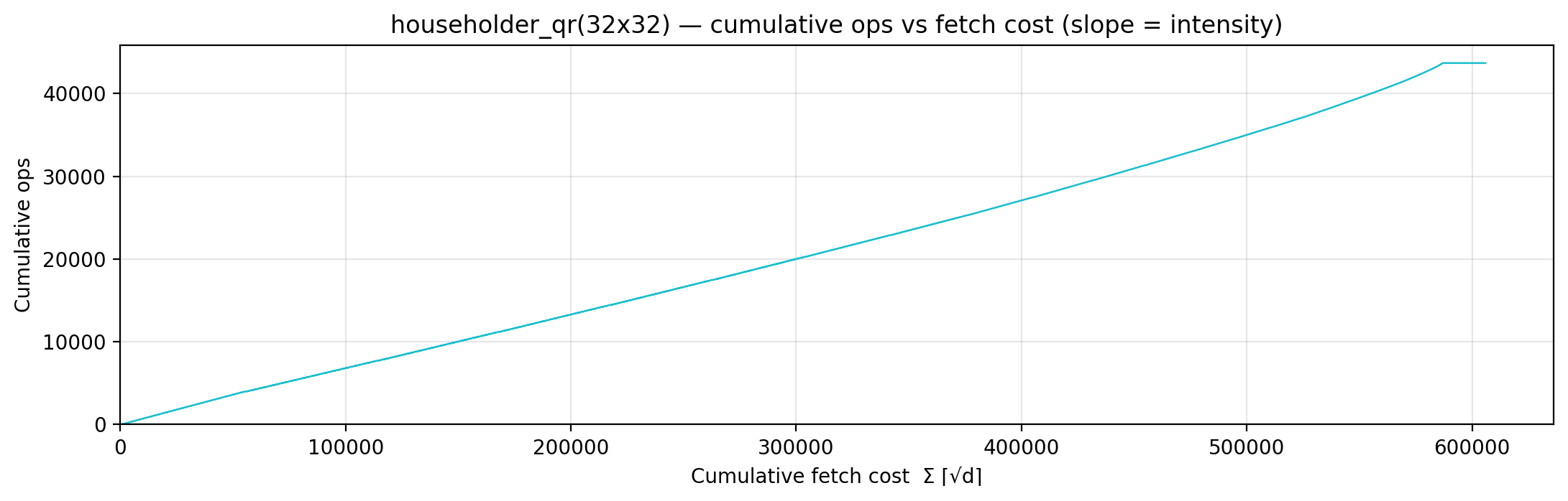
Gravity well — per-load fetch-cost ⌈√d⌉ scatter.
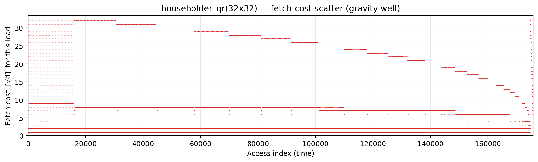
Spatial locality CDF — compute-fulfillment as a function of radius.
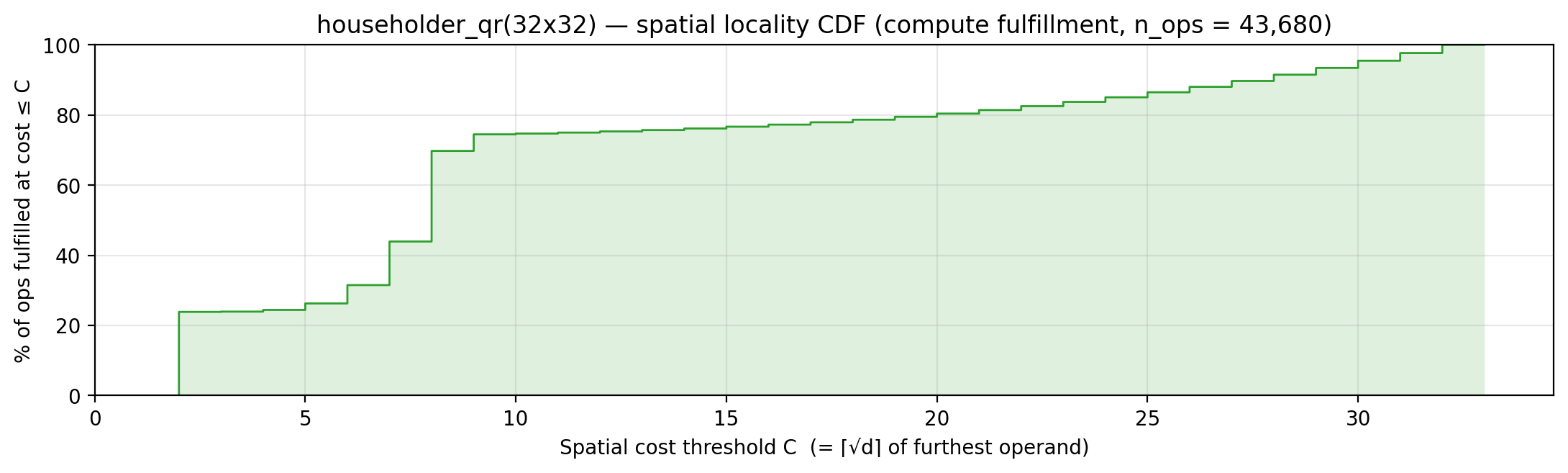
Working-set size over a τ = 428-event window (max = 428).
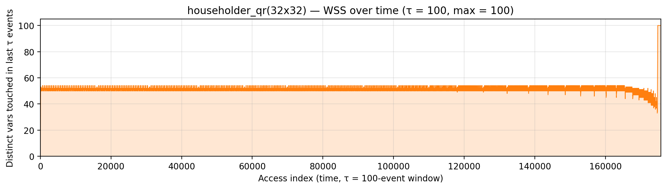
blocked_qr (code)
32×32, NB=8. Algorithm. WY-form block Householder (simplified):
factor an NB-column panel with classical Householder, then apply the
accumulated block reflector to the trailing columns in one
rank-NB sweep per column (compute NB-vector w = W^T · col, then
col -= V · w).
Manual placement. Three hoisted scratchpads at the bottom of the
stack, plus a loop restructure that pulls the trailing-panel update
into reflector-outer / column-inner order (valid because different
columns are independent):
c_A (addr 1) dot-product accumulator;
c_V (addrs 2..m+1) reflector column buffer, loaded once per k
and reused across all trailing j columns;
c_W (addrs m+2..m+NB+1) per-reflector dot cache for the
intra-panel update (was w).
Inner body now reads 1 bulk cell plus 2 hot scratchpad cells. Drops
manual from 1,175,373 to 762,199 (−35%), still above
global_density (476,803) because full WY factoring (accumulating
the V·T·Vᵀ block reflector) isn’t implemented.
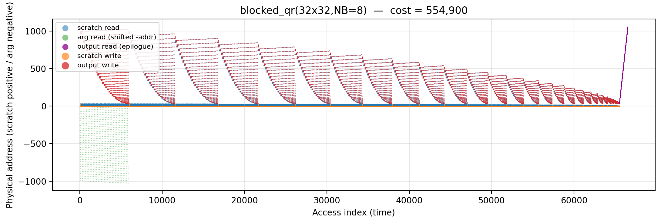
Working-set size over time (peak = 1,033).
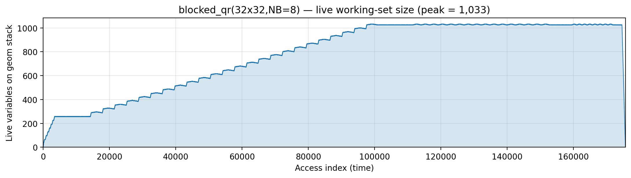
Reuse distance per load — LRU vs Bélády OPT (max LRU = 1,024; max OPT = 1,024).
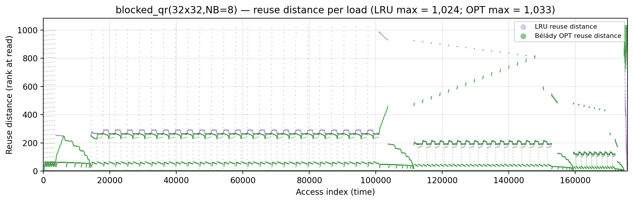
Miss-ratio curve — LRU vs Bélády OPT misses by cache capacity.
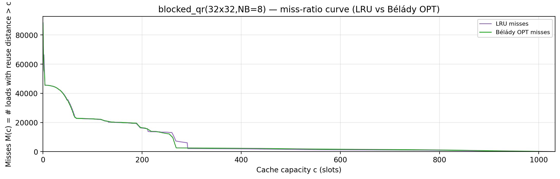
Per-tick TU LP floor — integrand of global_density: Σ_i ρ_{(i)} · √i over currently-live vars, ranked by density; the area equals global_density.

Per-tick splitting LP floor — integrand of local_density: Σ_i ρ_{(i)} · √i over the currently-active per-burst virtual intervals; the area equals the geometric portion of local_density.

Rolling spatial intensity — heartbeat plot of ops / Σ ⌈√d⌉ over a sliding window.
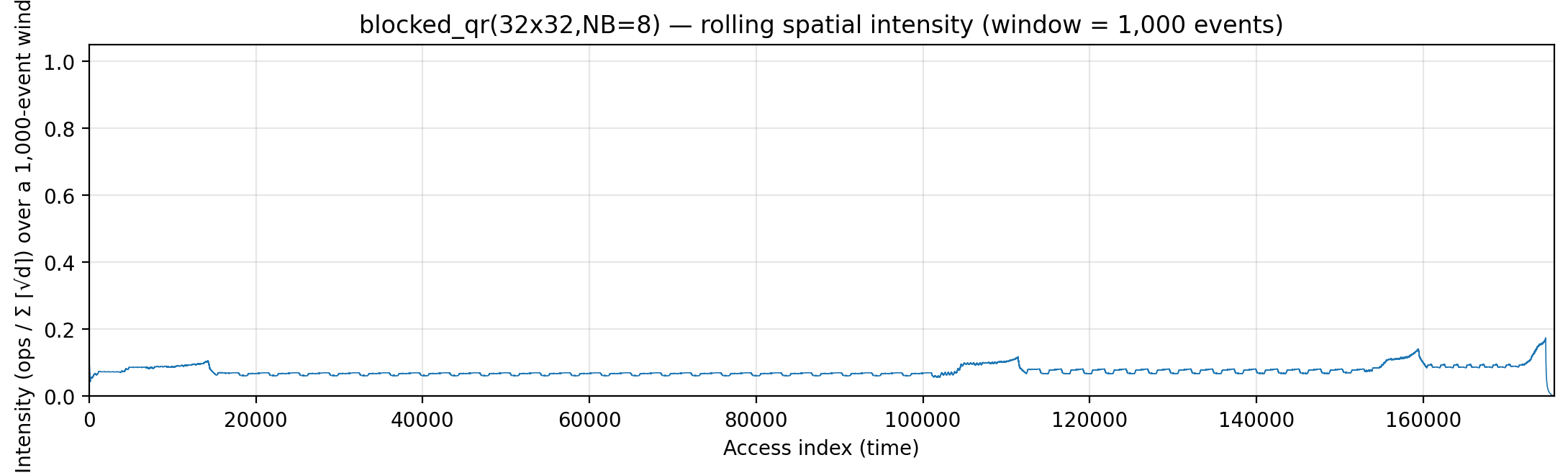
Cumulative compute vs fetch cost — slope = instantaneous spatial arithmetic intensity.
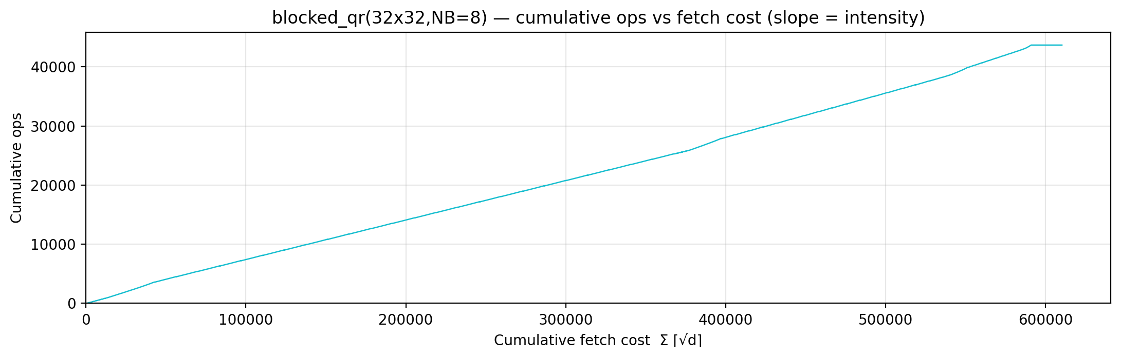
Gravity well — per-load fetch-cost ⌈√d⌉ scatter.
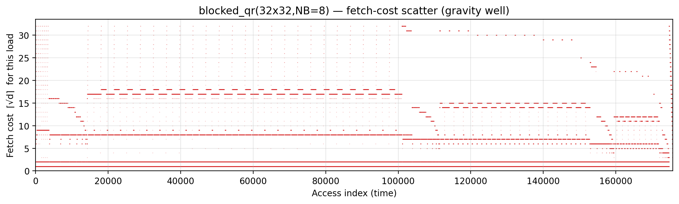
Spatial locality CDF — compute-fulfillment as a function of radius.
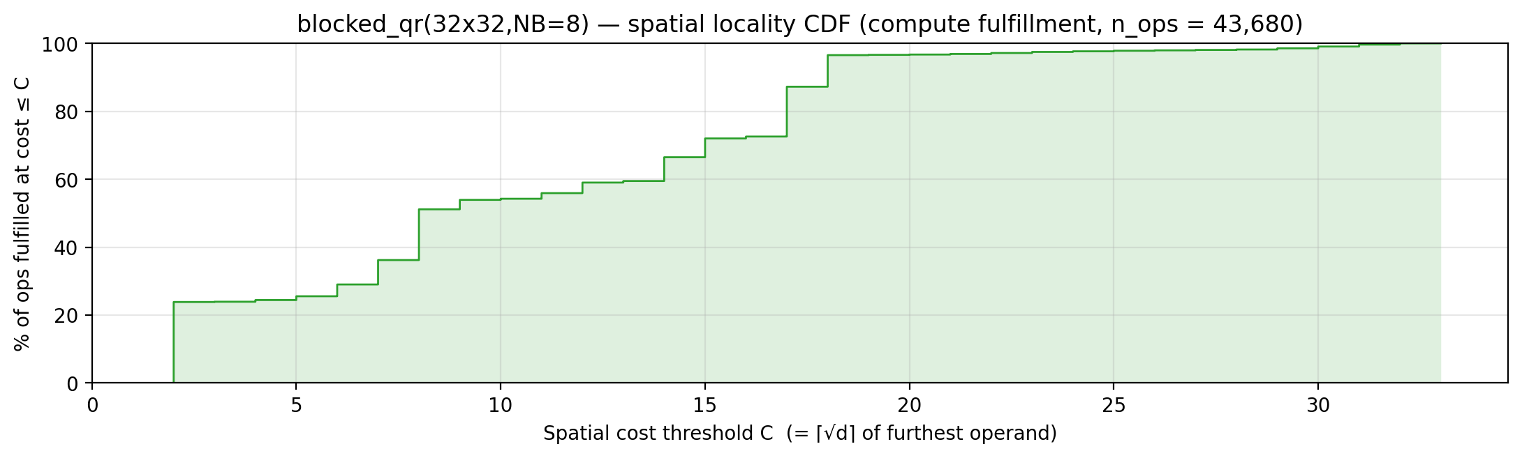
Working-set size over a τ = 267-event window (max = 267).
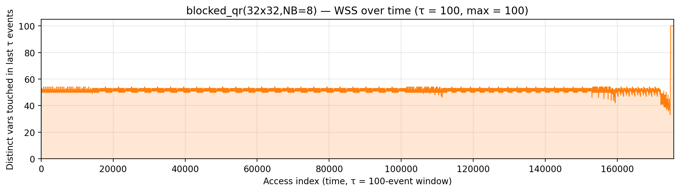
tsqr (code)
64×16, block_rows=8. Algorithm. Communication-avoiding TSQR:
split the tall 64×16 matrix into 8 row-tiles of 8 rows; factor each
tile independently with local Householder QR; merge the resulting R
factors pairwise up a binary tree (log₂(#tiles) levels of
reductions).
Manual placement. Three stacked optimizations (gemini/optimize-tsqr.md):
- L1 tile funnel
cache_A— the current row-tile (block_rows×n = 128 cells) lives in a scratchpad at the very bottom of the stack. All Phase-1 inner-loop reads hit these low addresses. - Asymmetric caching in Phase 2 — only the right R-factor block is
pulled into
cache_A; the left block’s sparsely-accessed k-th row reads come directly from A (and the frequency-ordered layout makes them cheap too). - Frequency-ordered layout — a dry-run counts per-cell touches
across both phases + epilogue; A and
cache_Athen pack the busiest cells at the lowest addresses (same trick as floyd_warshall_recursive and recursive_lu).
Drops manual from 461,782 to 297,513 (−36%), within ~10% of
bytedmd_live (267,962).
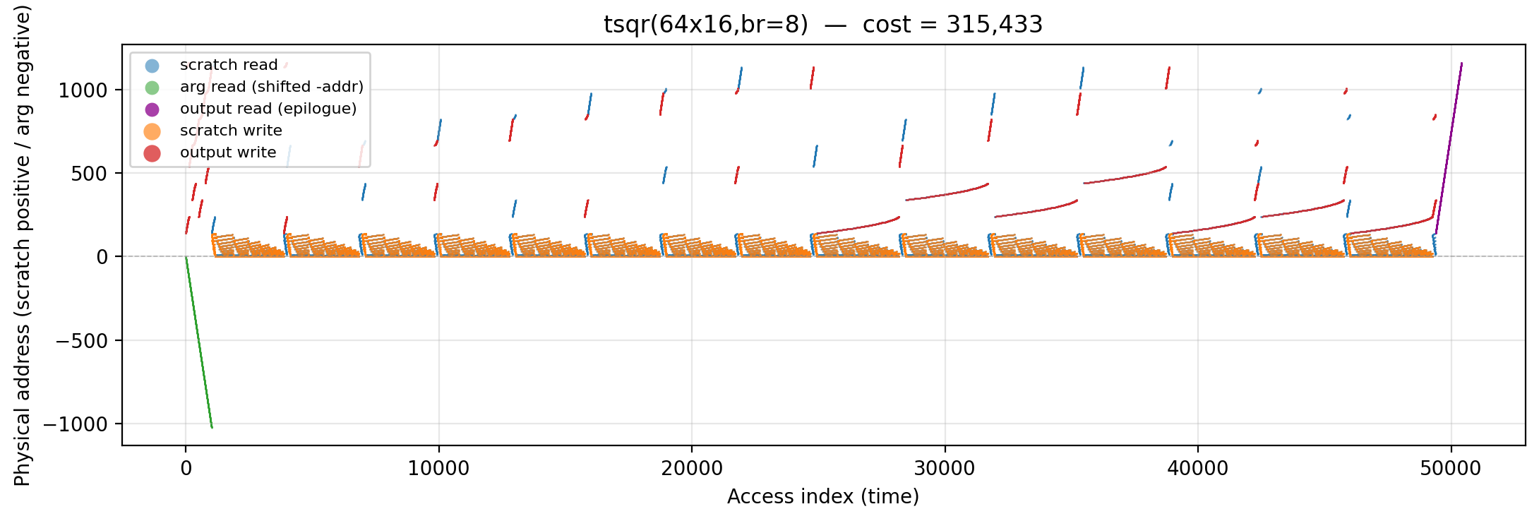
Working-set size over time (peak = 1,026).
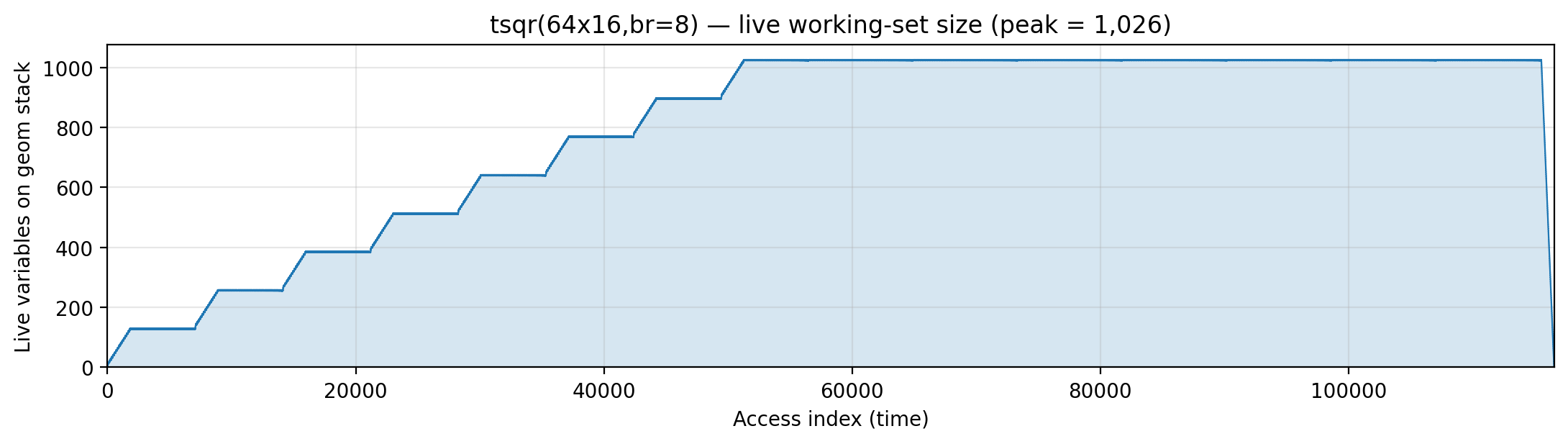
Reuse distance per load — LRU vs Bélády OPT (max LRU = 1,024; max OPT = 1,024).
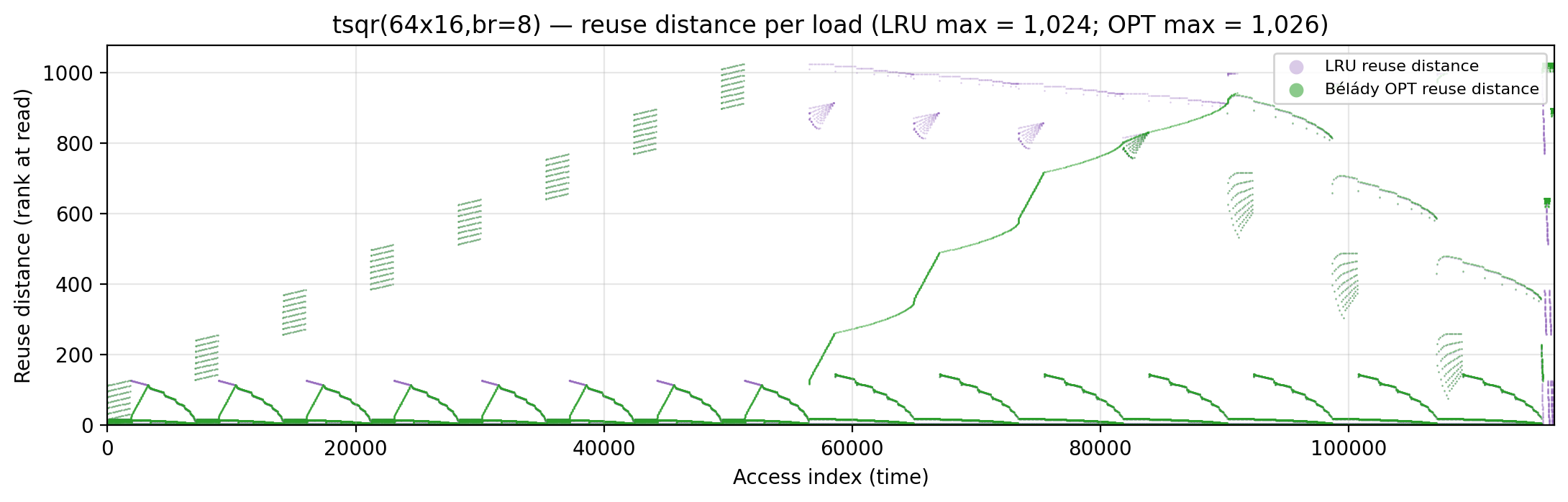
Miss-ratio curve — LRU vs Bélády OPT misses by cache capacity.
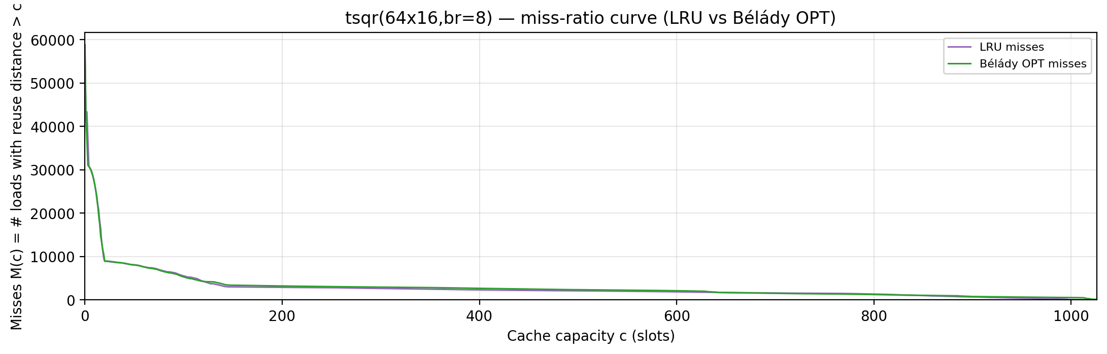
Per-tick TU LP floor — integrand of global_density: Σ_i ρ_{(i)} · √i over currently-live vars, ranked by density; the area equals global_density.
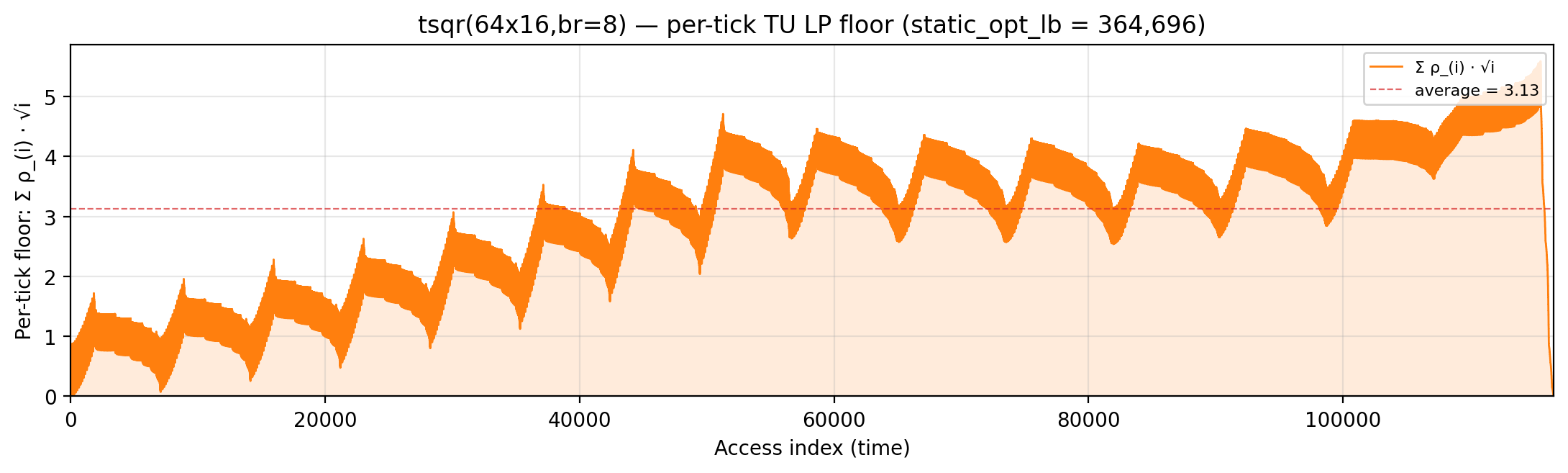
Per-tick splitting LP floor — integrand of local_density: Σ_i ρ_{(i)} · √i over the currently-active per-burst virtual intervals; the area equals the geometric portion of local_density.
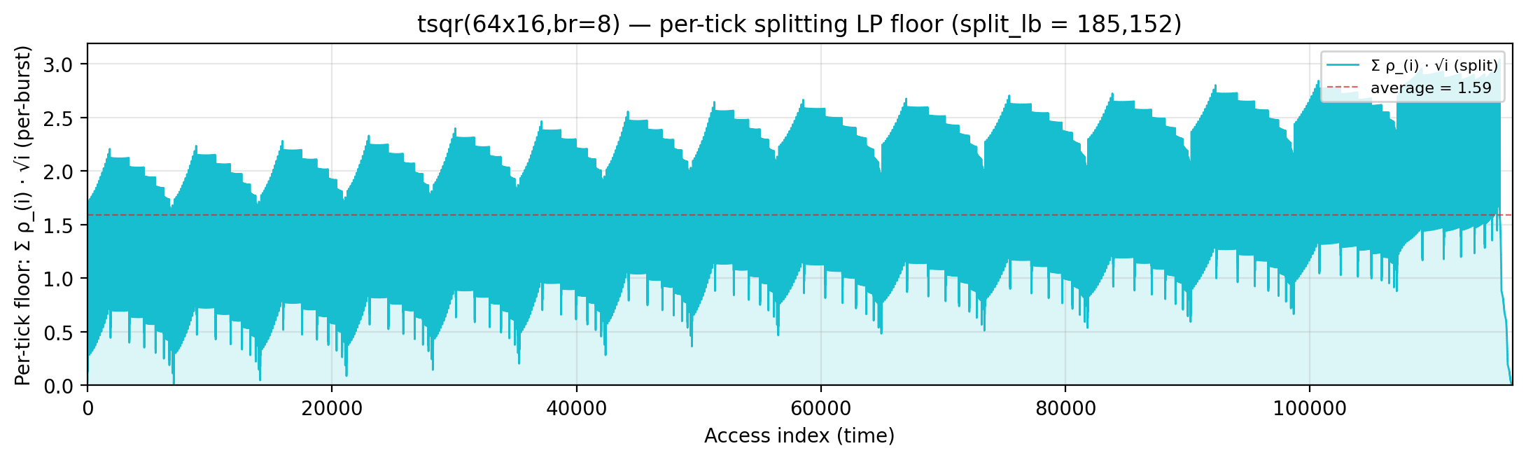
Rolling spatial intensity — heartbeat plot of ops / Σ ⌈√d⌉ over a sliding window.
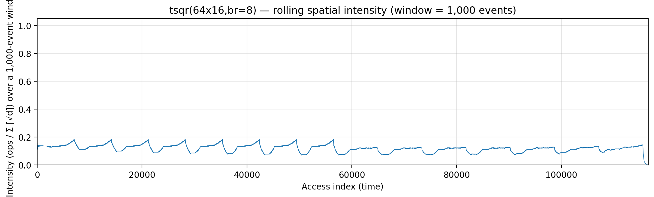
Cumulative compute vs fetch cost — slope = instantaneous spatial arithmetic intensity.
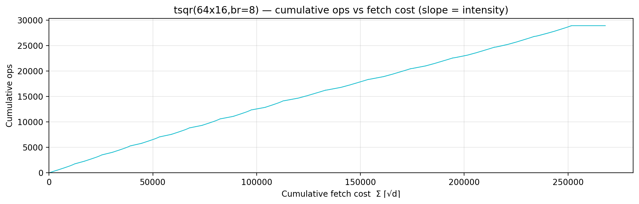
Gravity well — per-load fetch-cost ⌈√d⌉ scatter.
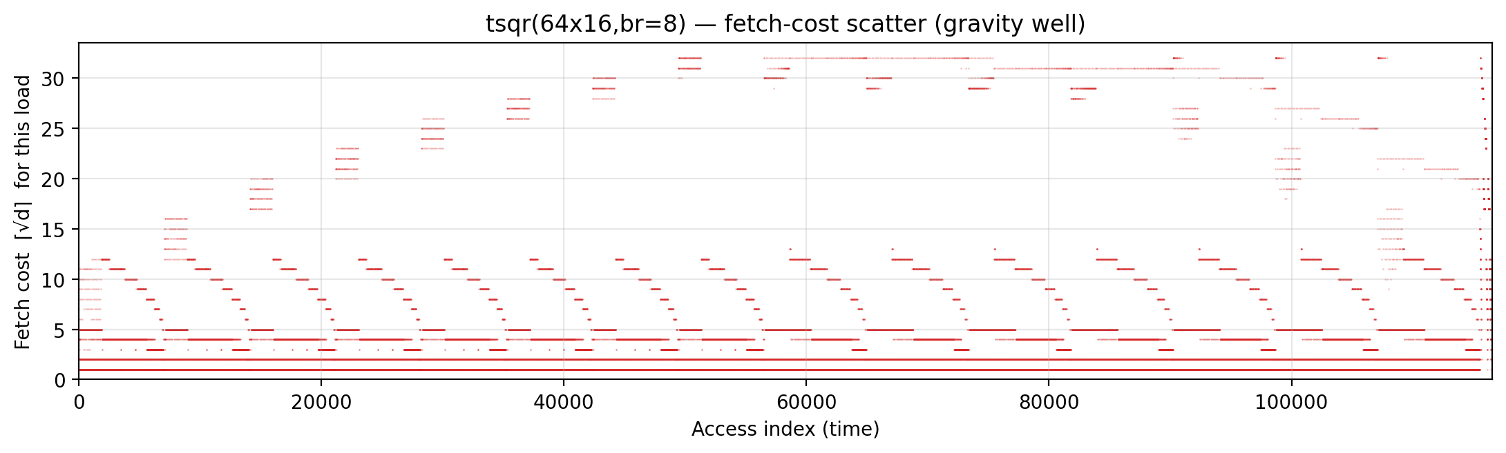
Spatial locality CDF — compute-fulfillment as a function of radius.
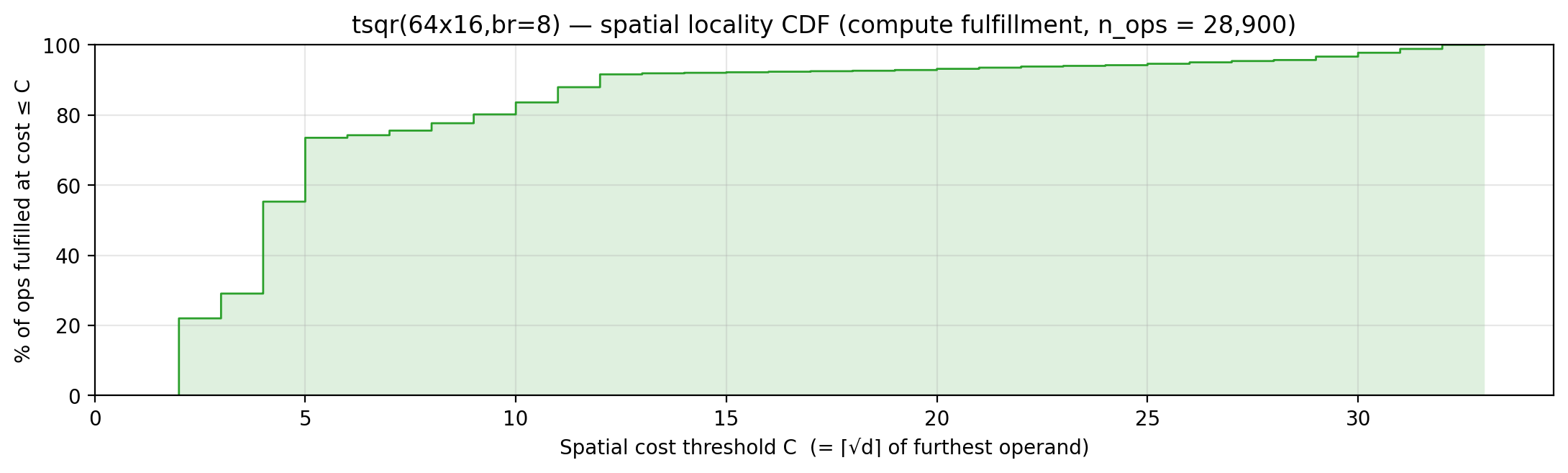
Working-set size over a τ = 96-event window (max = 96).
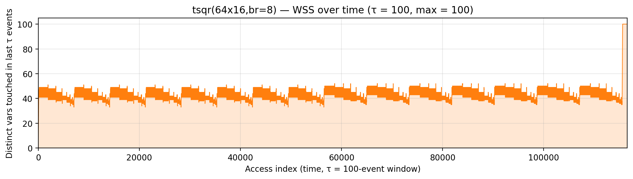
transpose_naive (code)
n=32. Algorithm. B[i][j] = A[j][i] read column-major. The cache-thrashing baseline — every A-read jumps by n bytes.
Manual placement. A on arg stack, B on scratch; the per-cell arg-read cost dominates.
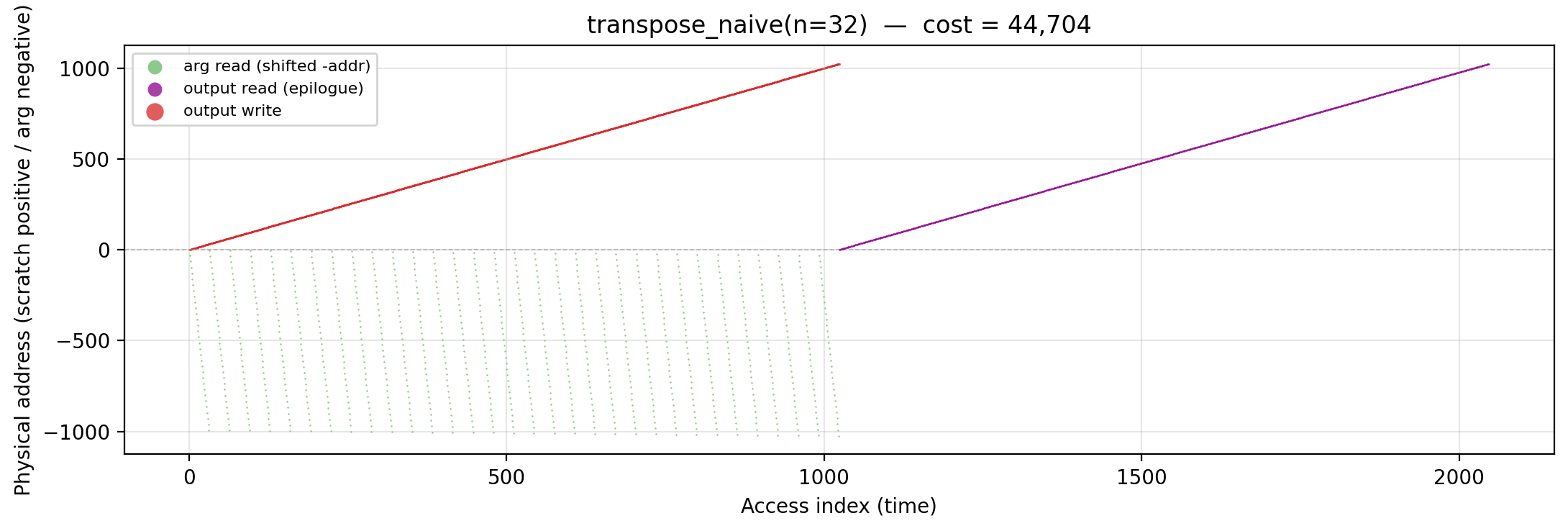
Working-set size over time (peak = 1,024).
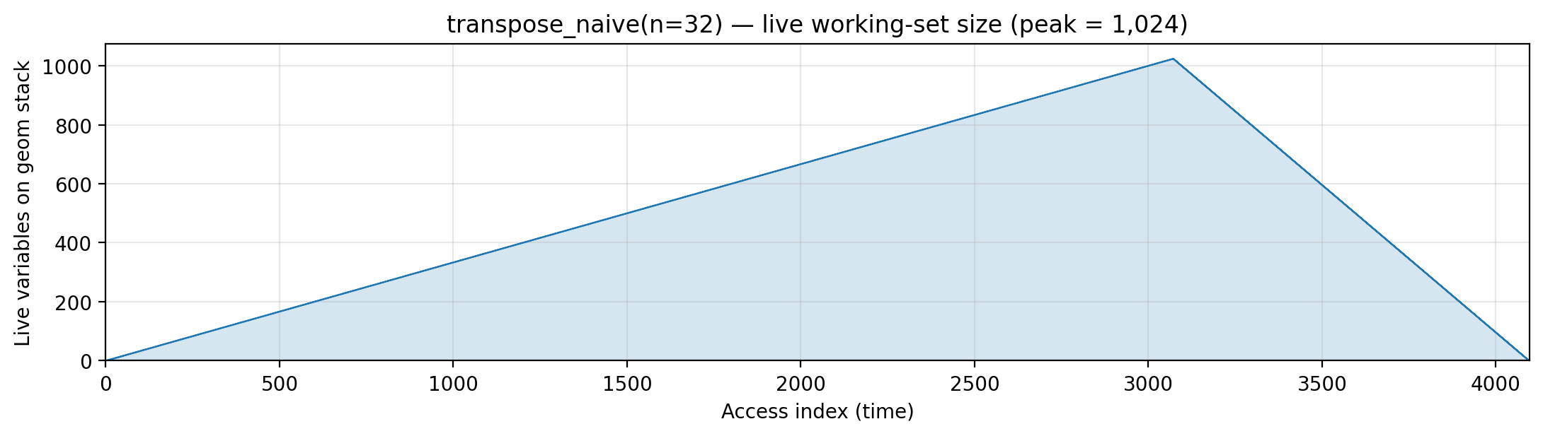
Reuse distance per load — LRU vs Bélády OPT (max LRU = 1,024; max OPT = 1,024).
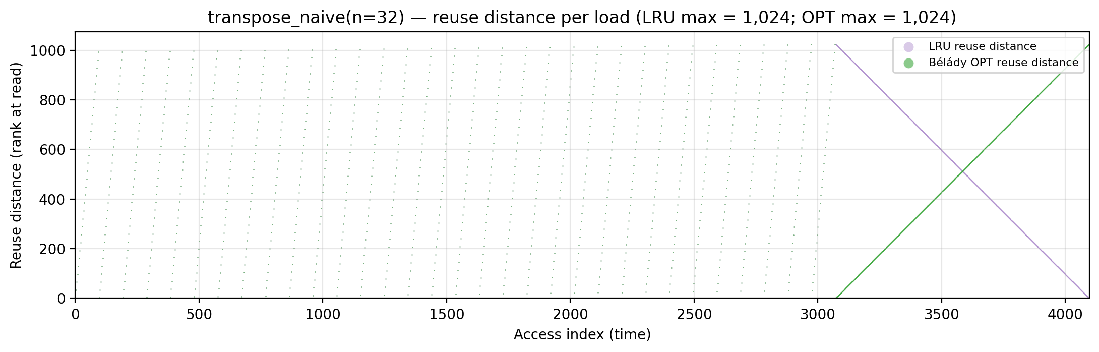
Miss-ratio curve — LRU vs Bélády OPT misses by cache capacity.
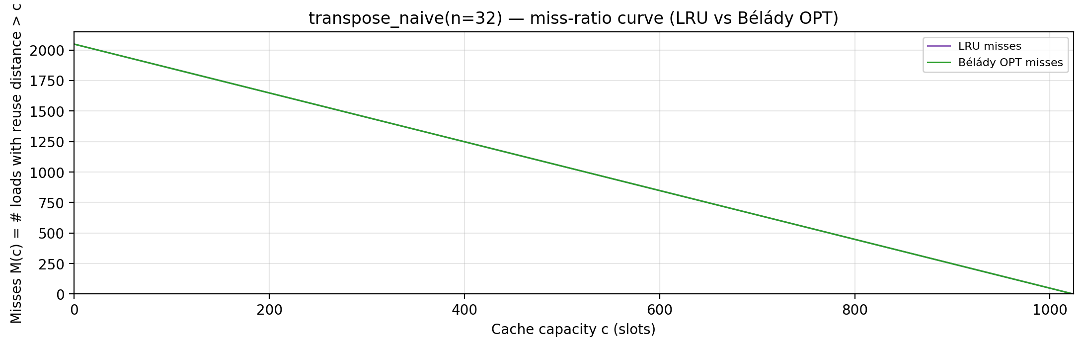
Per-tick TU LP floor — integrand of global_density: Σ_i ρ_{(i)} · √i over currently-live vars, ranked by density; the area equals global_density.
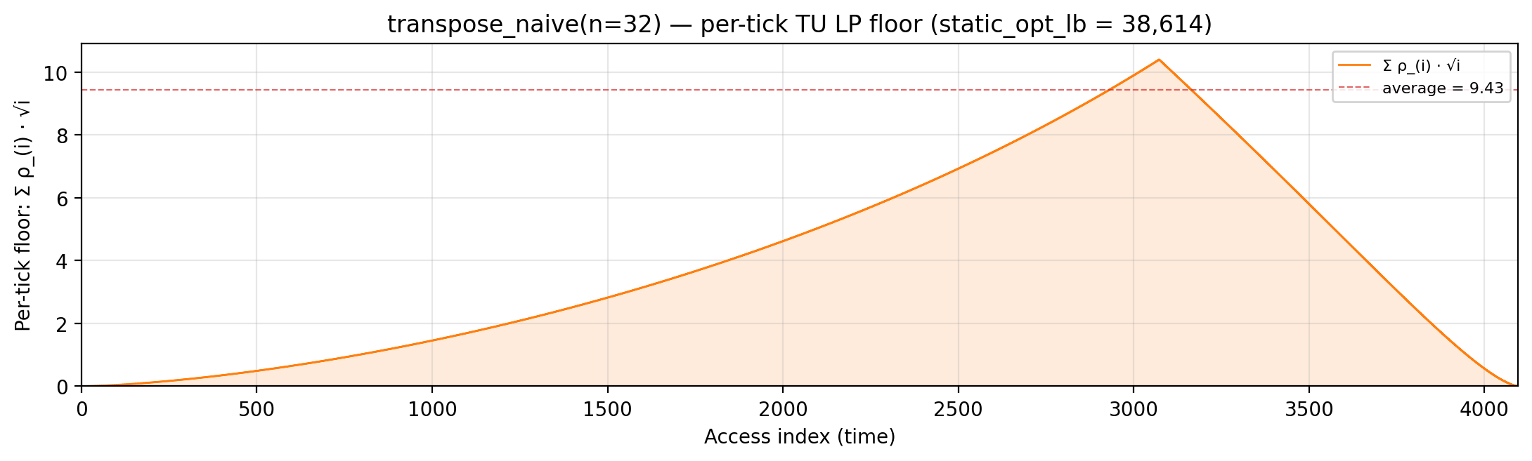
Per-tick splitting LP floor — integrand of local_density: Σ_i ρ_{(i)} · √i over the currently-active per-burst virtual intervals; the area equals the geometric portion of local_density.
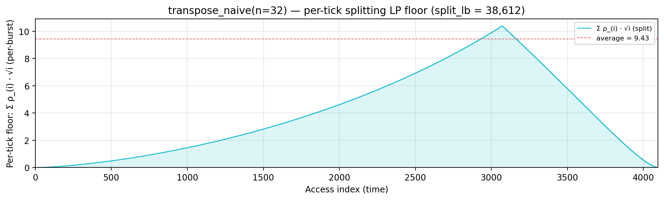
Rolling spatial intensity — heartbeat plot of ops / Σ ⌈√d⌉ over a sliding window.
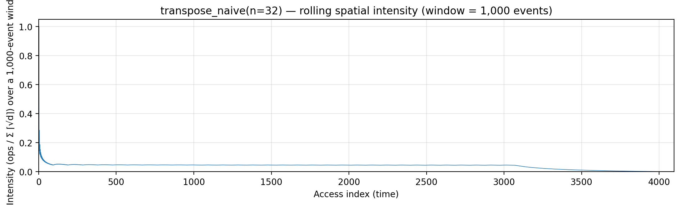
Cumulative compute vs fetch cost — slope = instantaneous spatial arithmetic intensity.
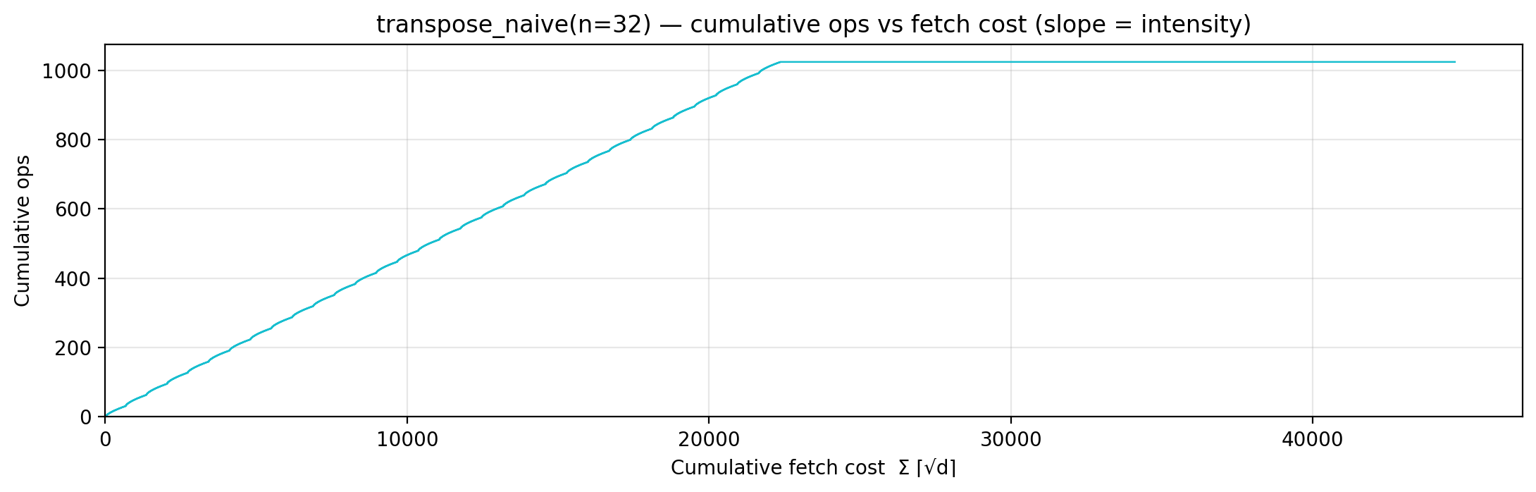
Gravity well — per-load fetch-cost ⌈√d⌉ scatter.
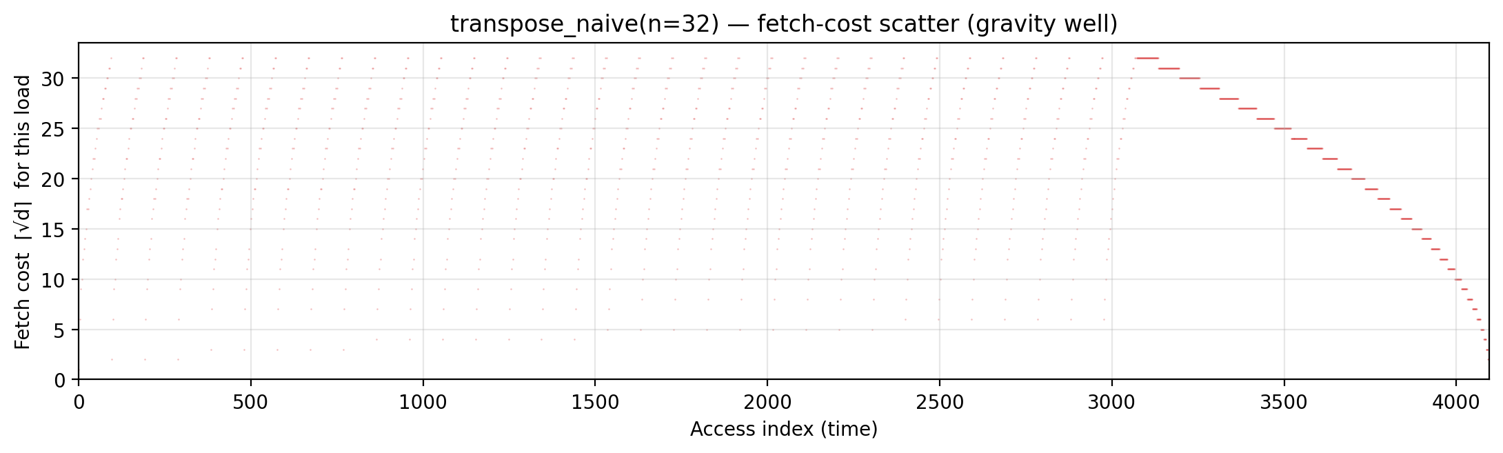
Spatial locality CDF — compute-fulfillment as a function of radius.
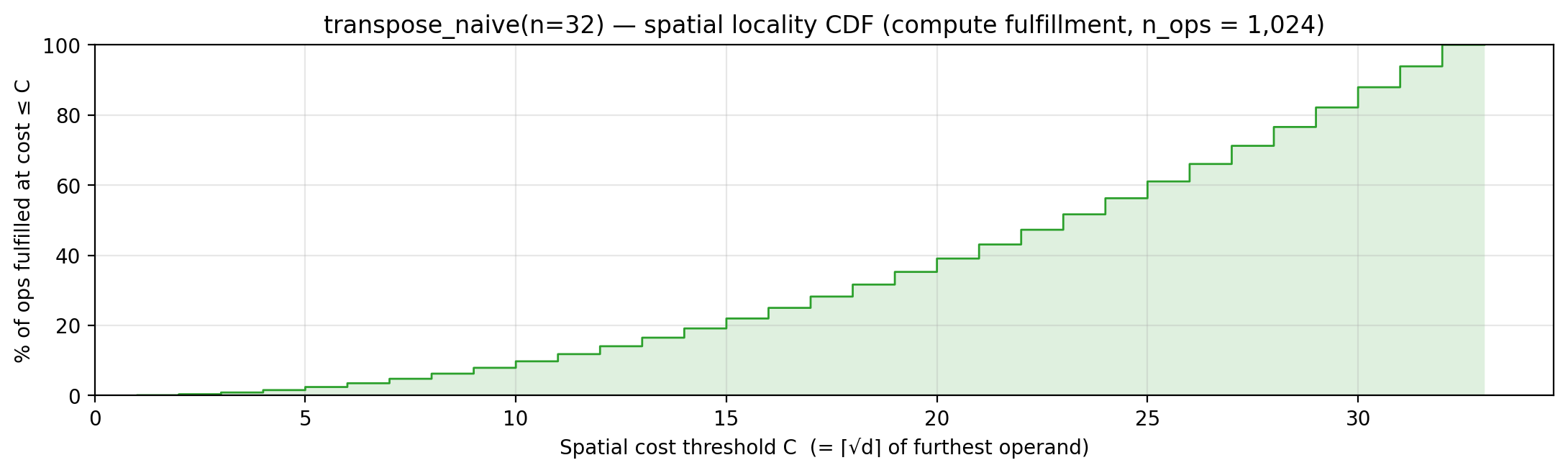
Working-set size over a τ = 922-event window (max = 922).
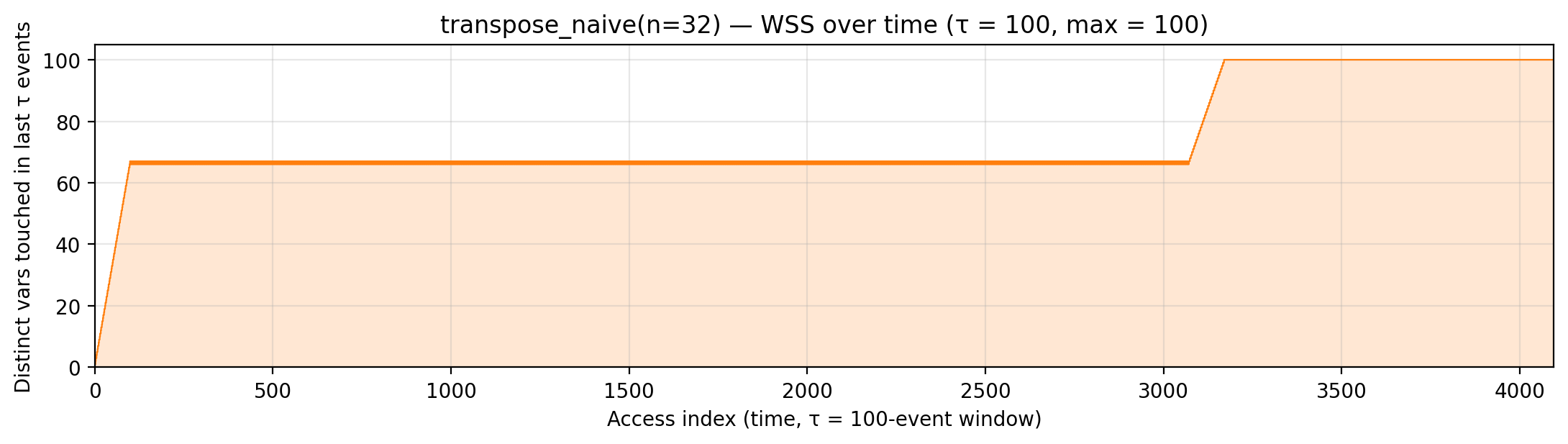
transpose_blocked (code)
n=32, T=√n. Algorithm. Blocked iteration over A — same reads as naive in block-major order.
Manual matches naive layout; the heuristics reward the locality-friendly order only where LRU recency and density ranking can catch it.
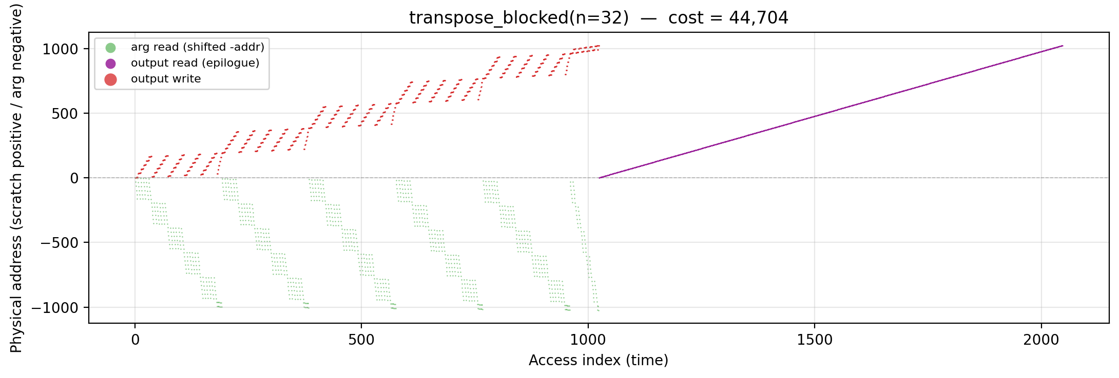
Working-set size over time (peak = 1,024).
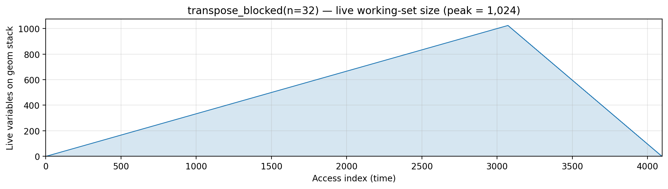
Reuse distance per load — LRU vs Bélády OPT (max LRU = 1,024; max OPT = 1,024).
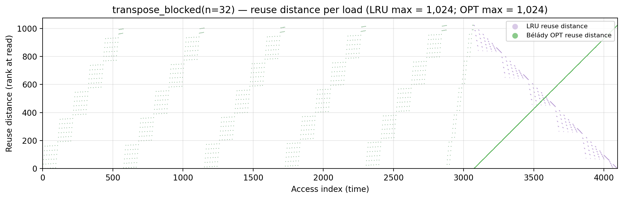
Miss-ratio curve — LRU vs Bélády OPT misses by cache capacity.
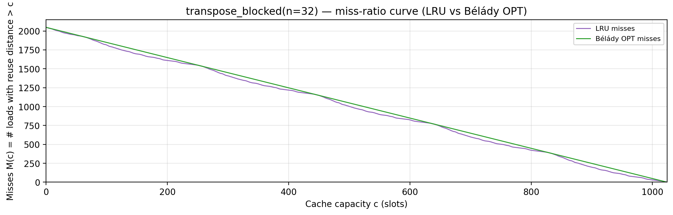
Per-tick TU LP floor — integrand of global_density: Σ_i ρ_{(i)} · √i over currently-live vars, ranked by density; the area equals global_density.
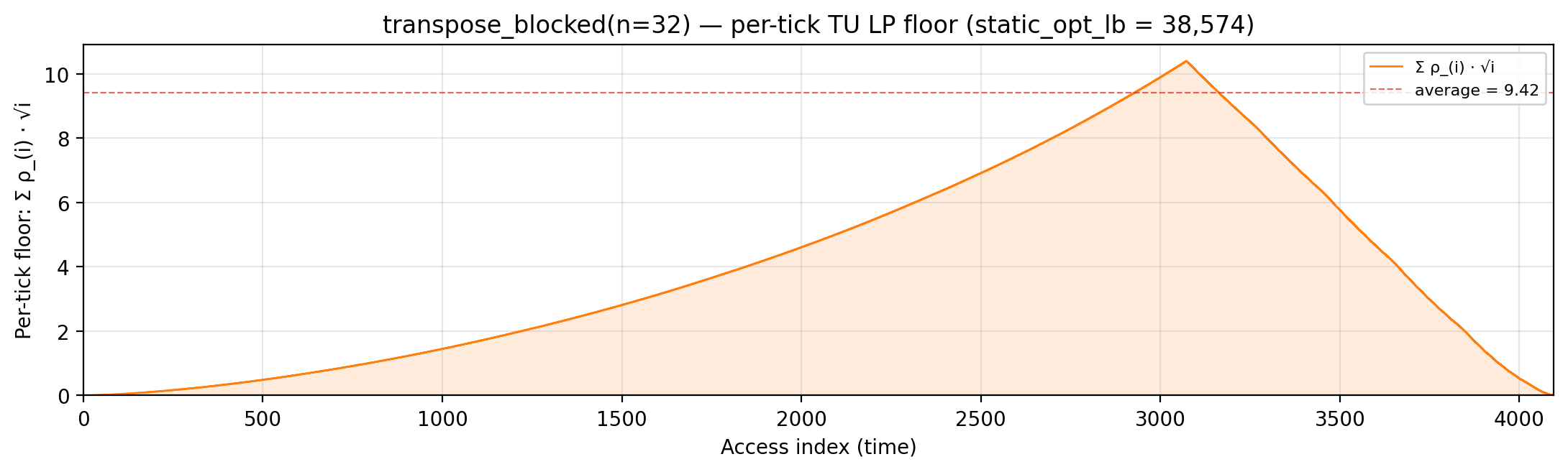
Per-tick splitting LP floor — integrand of local_density: Σ_i ρ_{(i)} · √i over the currently-active per-burst virtual intervals; the area equals the geometric portion of local_density.
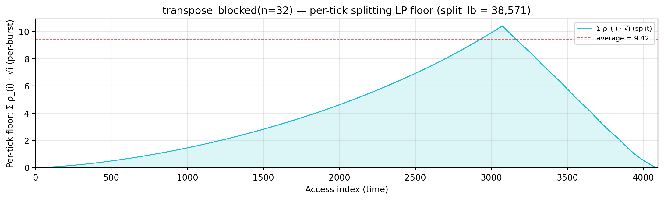
Rolling spatial intensity — heartbeat plot of ops / Σ ⌈√d⌉ over a sliding window.
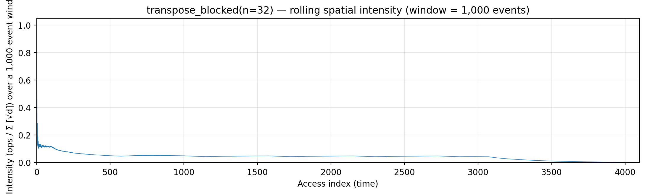
Cumulative compute vs fetch cost — slope = instantaneous spatial arithmetic intensity.
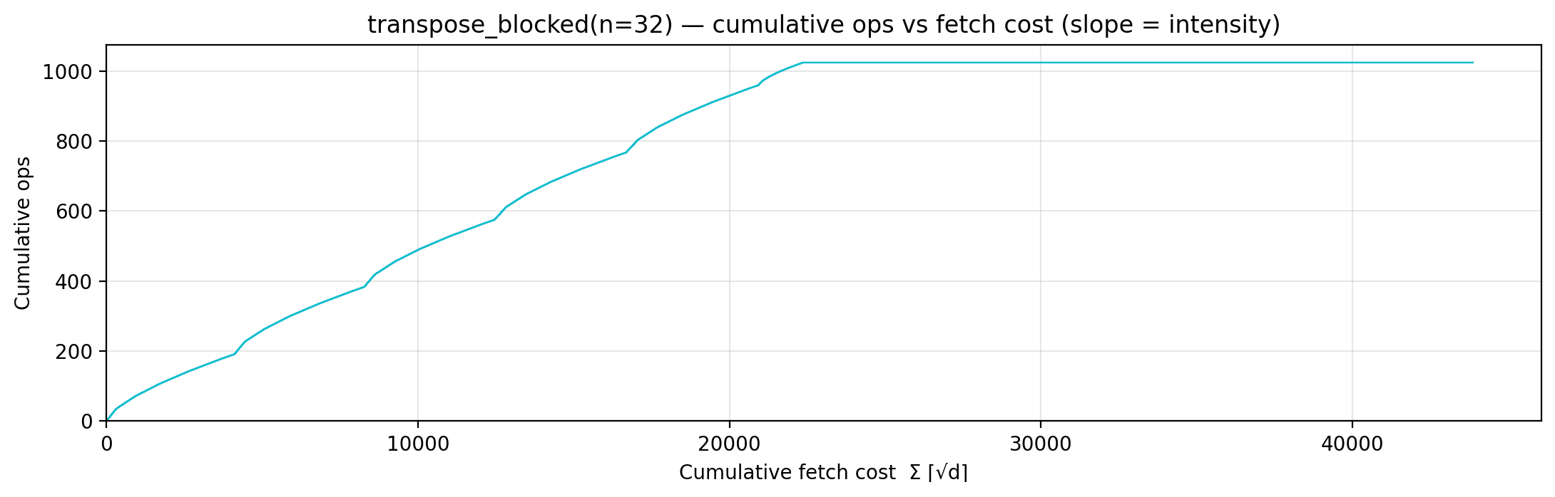
Gravity well — per-load fetch-cost ⌈√d⌉ scatter.
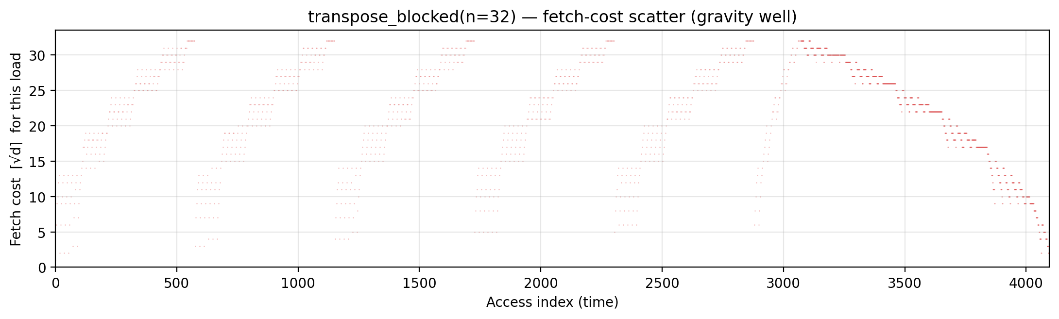
Spatial locality CDF — compute-fulfillment as a function of radius.
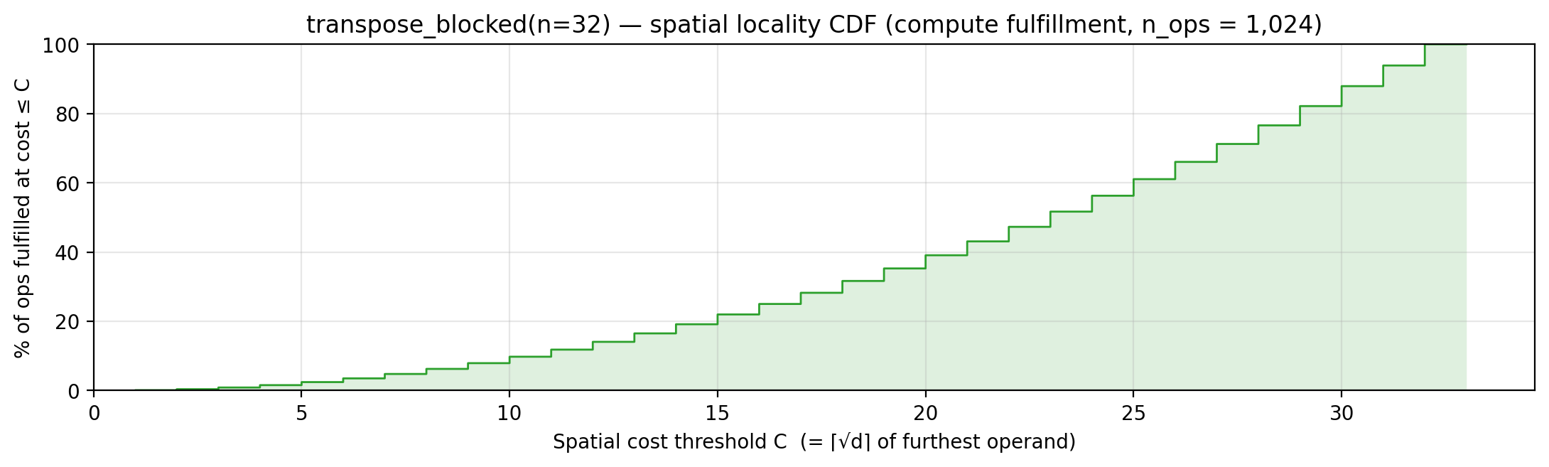
Working-set size over a τ = 897-event window (max = 897).
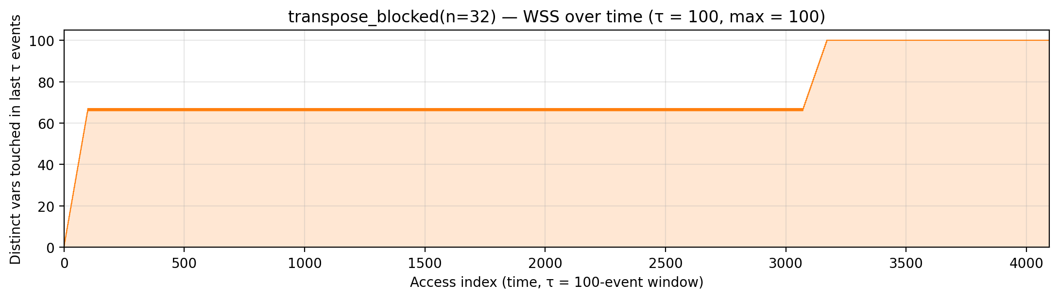
transpose_recursive (code)
n=32. Algorithm. Cache-oblivious recursive transpose — split into 4 quadrants until sz=1.
Manual again matches the same fixed A/B addresses; heuristic difference comes from the quadrant traversal order.
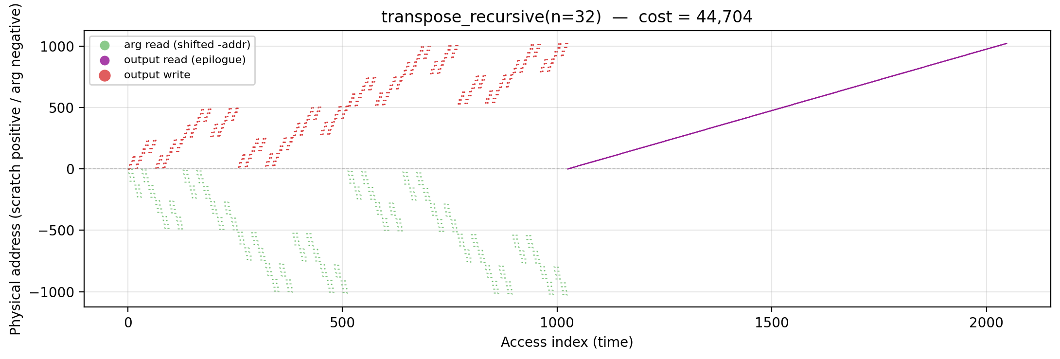
Working-set size over time (peak = 1,024).
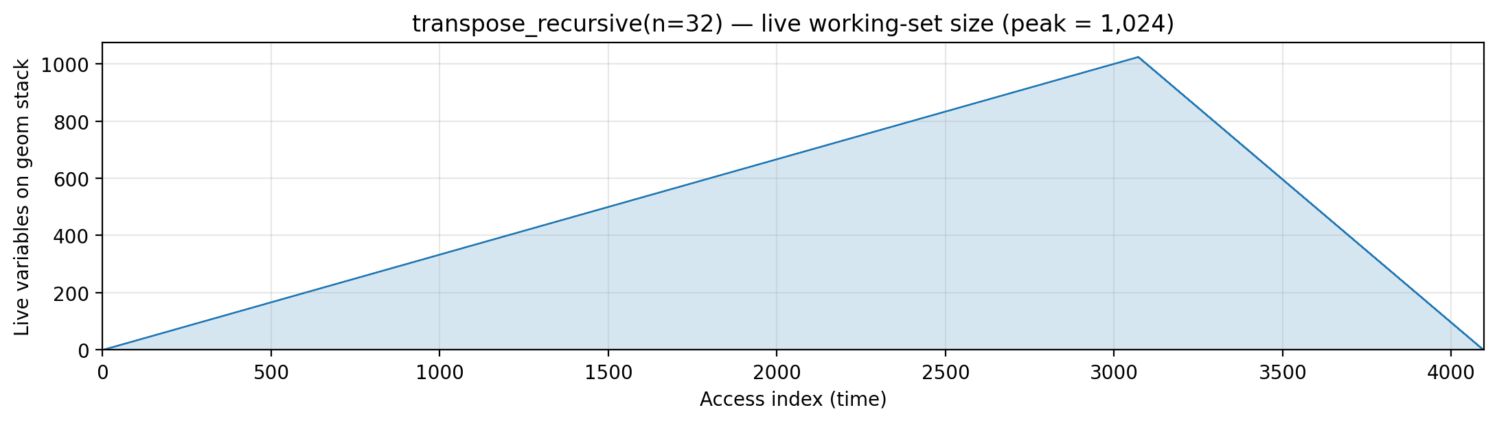
Reuse distance per load — LRU vs Bélády OPT (max LRU = 1,024; max OPT = 1,024).
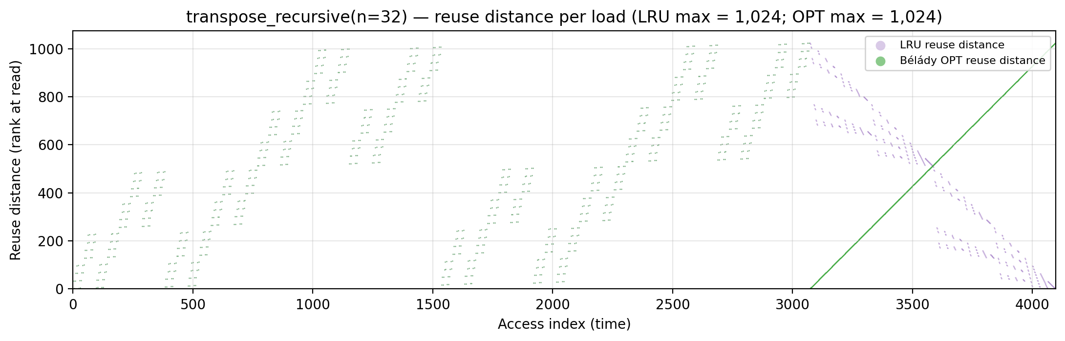
Miss-ratio curve — LRU vs Bélády OPT misses by cache capacity.
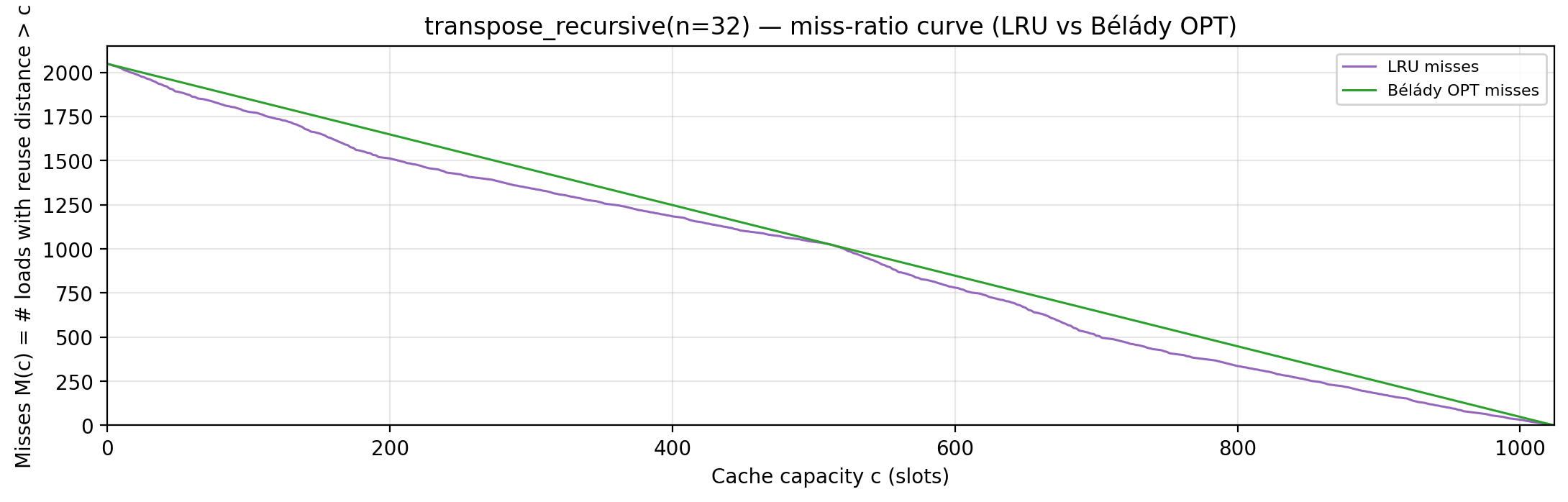
Per-tick TU LP floor — integrand of global_density: Σ_i ρ_{(i)} · √i over currently-live vars, ranked by density; the area equals global_density.
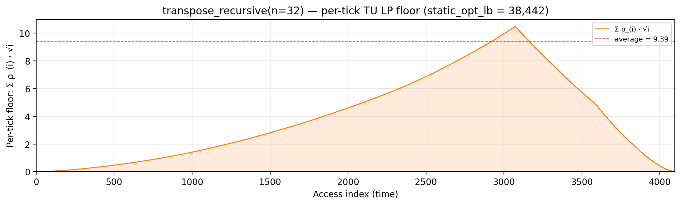
Per-tick splitting LP floor — integrand of local_density: Σ_i ρ_{(i)} · √i over the currently-active per-burst virtual intervals; the area equals the geometric portion of local_density.
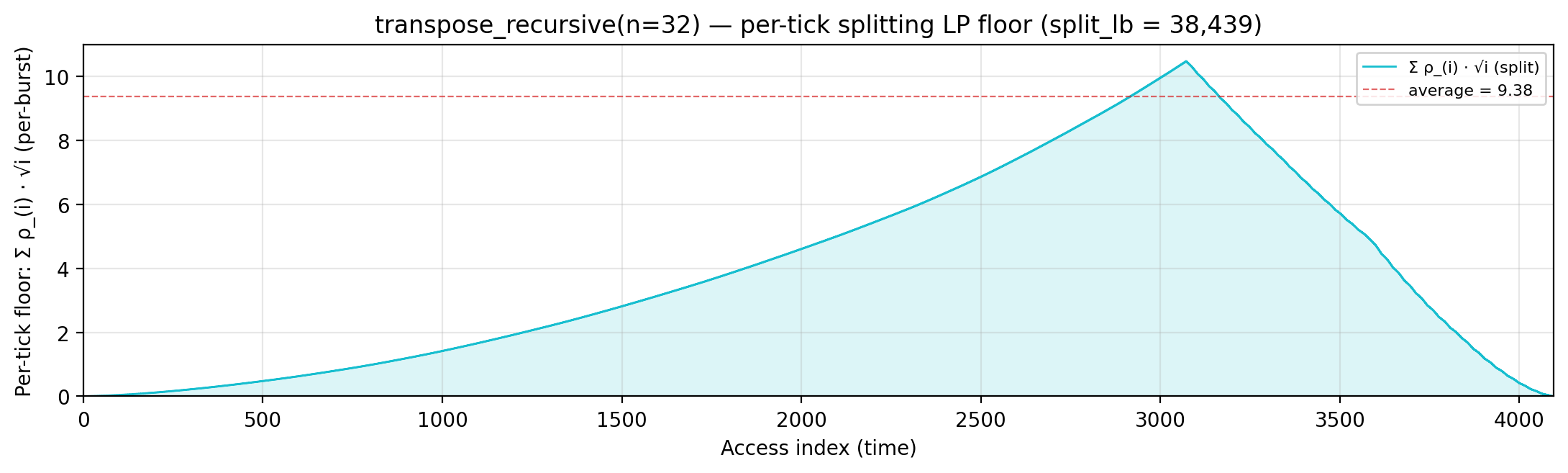
Rolling spatial intensity — heartbeat plot of ops / Σ ⌈√d⌉ over a sliding window.
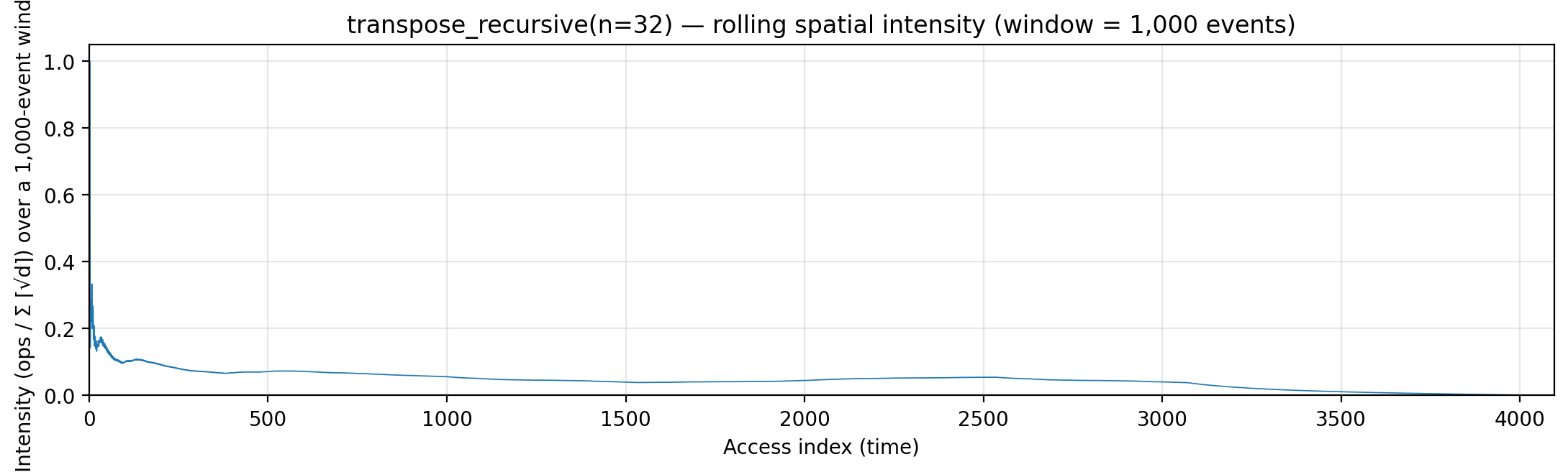
Cumulative compute vs fetch cost — slope = instantaneous spatial arithmetic intensity.
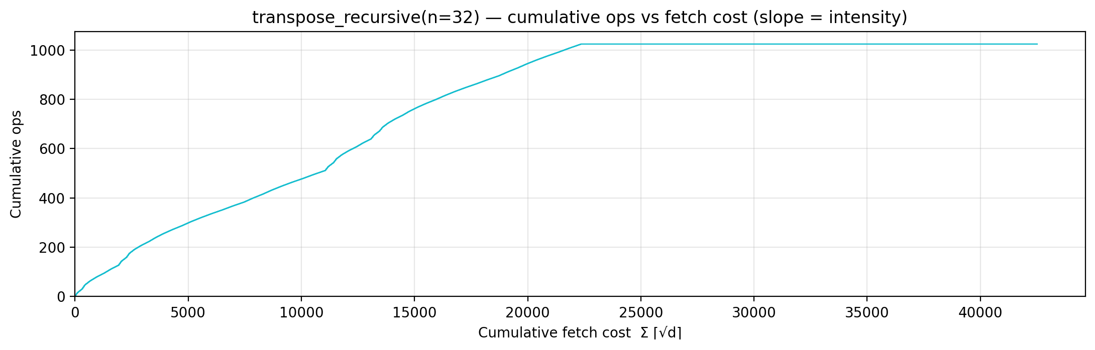
Gravity well — per-load fetch-cost ⌈√d⌉ scatter.
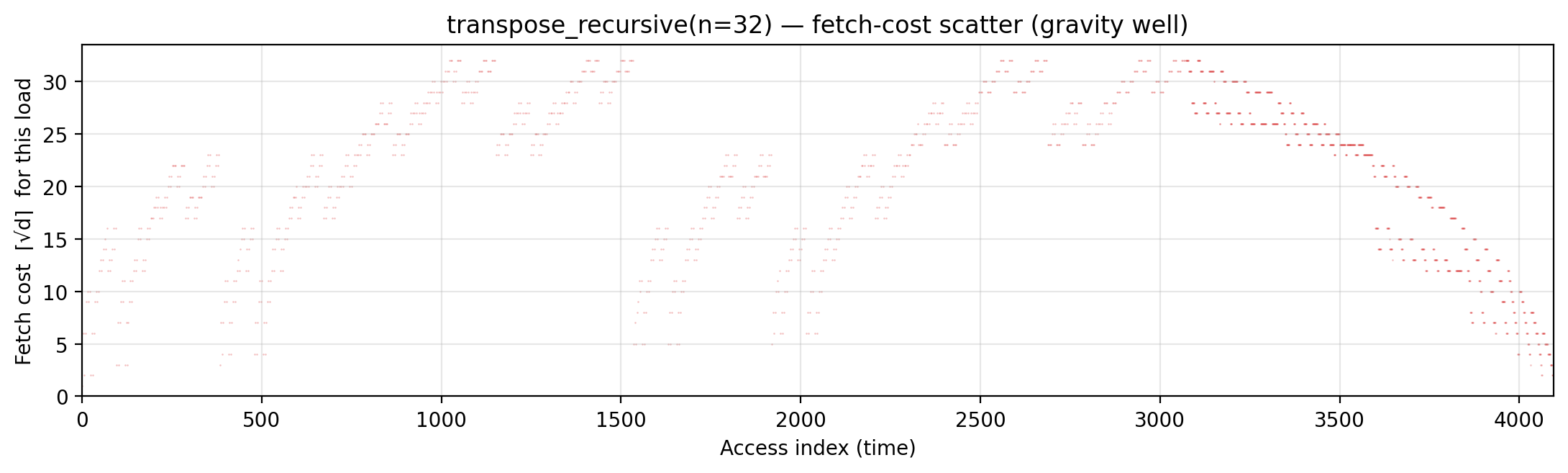
Spatial locality CDF — compute-fulfillment as a function of radius.
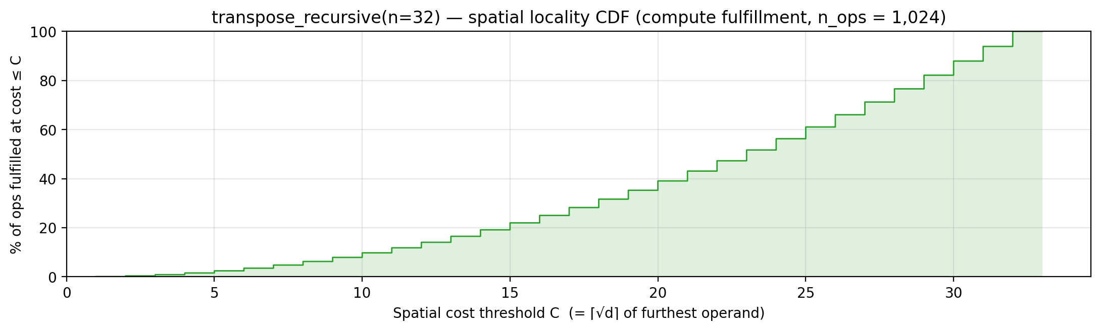
Working-set size over a τ = 884-event window (max = 884).
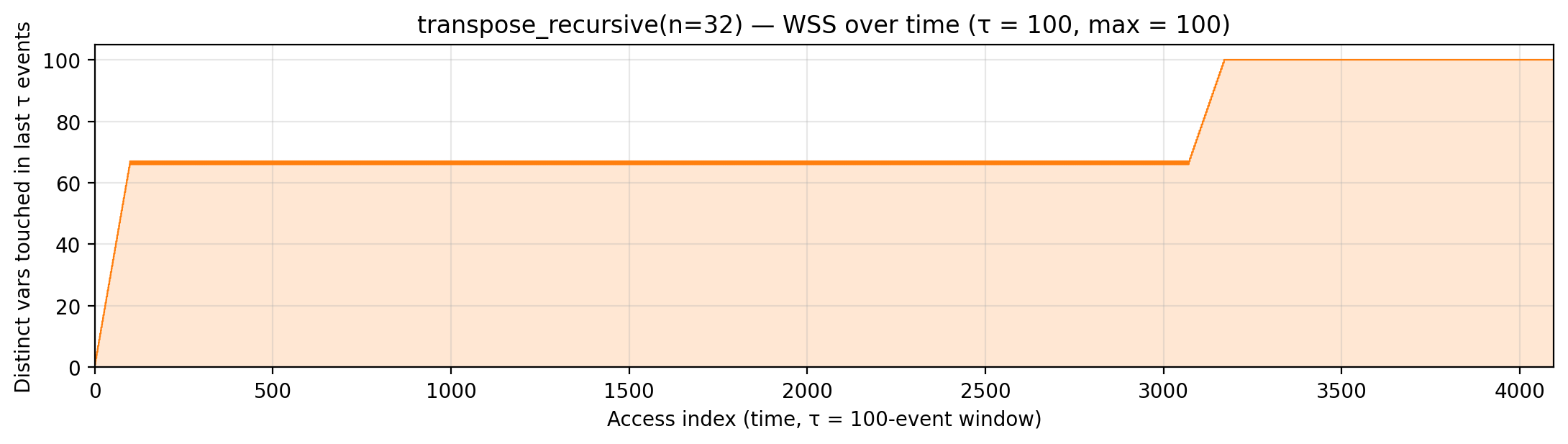
stencil_time_naive (code)
n=16, T=4. Algorithm. 4 full Jacobi sweeps, each reading the current grid and writing a fresh next-timestep buffer — naive communication-avoiding baseline.
Manual. Input A preloaded to scratch cur, ping-pong with nxt. Every cell is re-touched T times from bulk scratch.
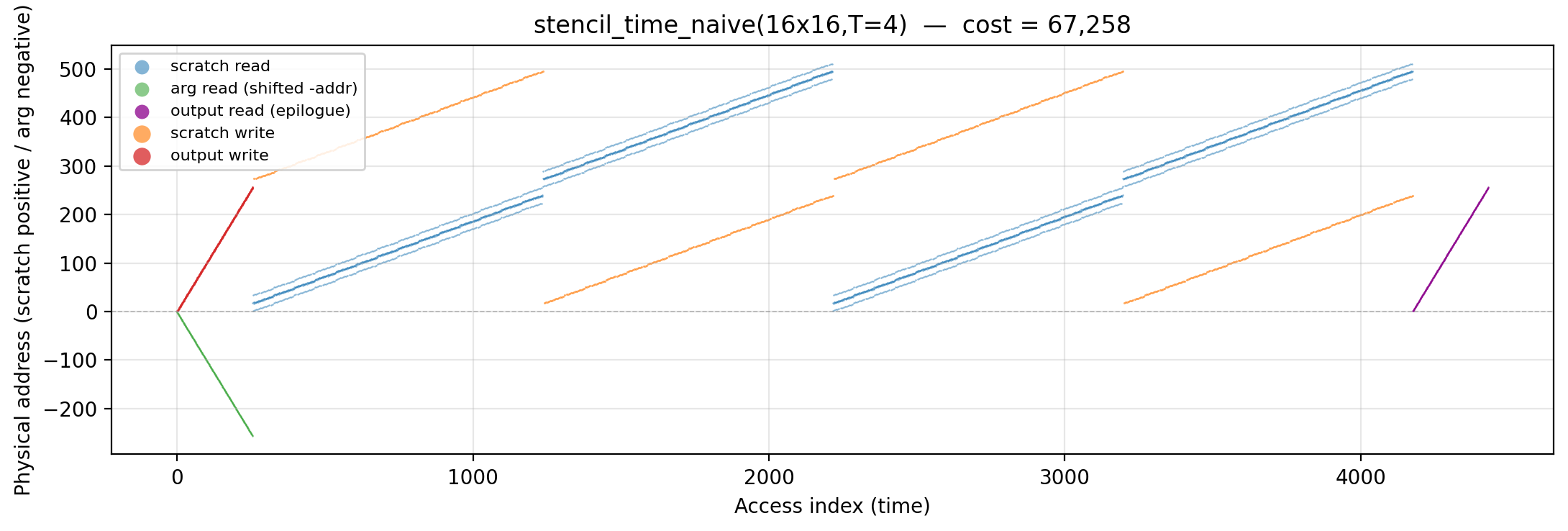
Working-set size over time (peak = 312).
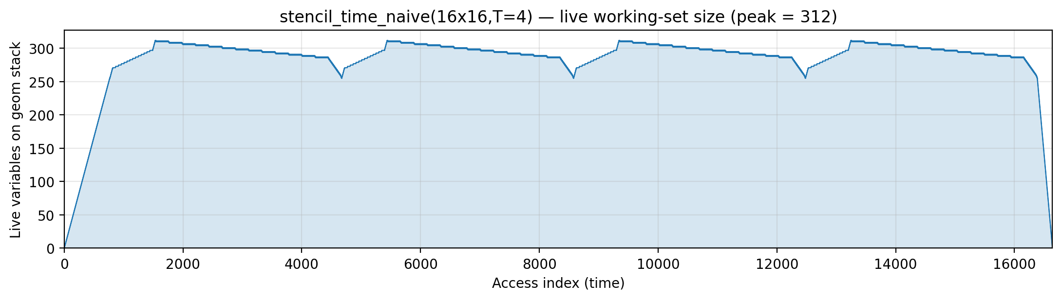
Reuse distance per load — LRU vs Bélády OPT (max LRU = 312; max OPT = 256).
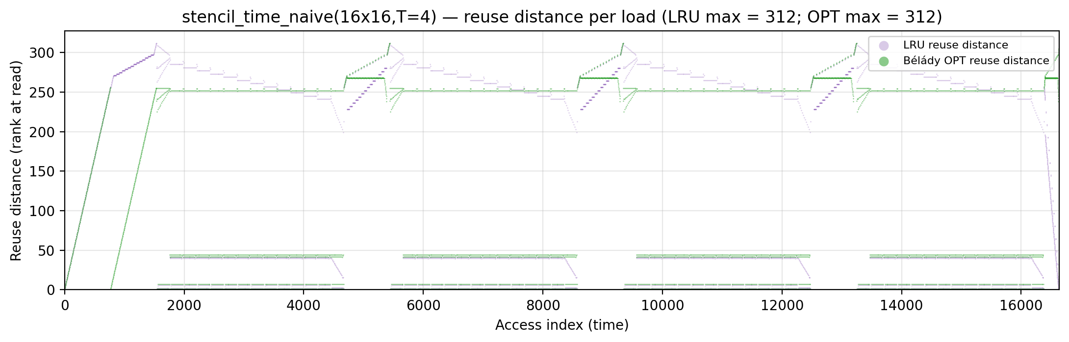
Miss-ratio curve — LRU vs Bélády OPT misses by cache capacity.
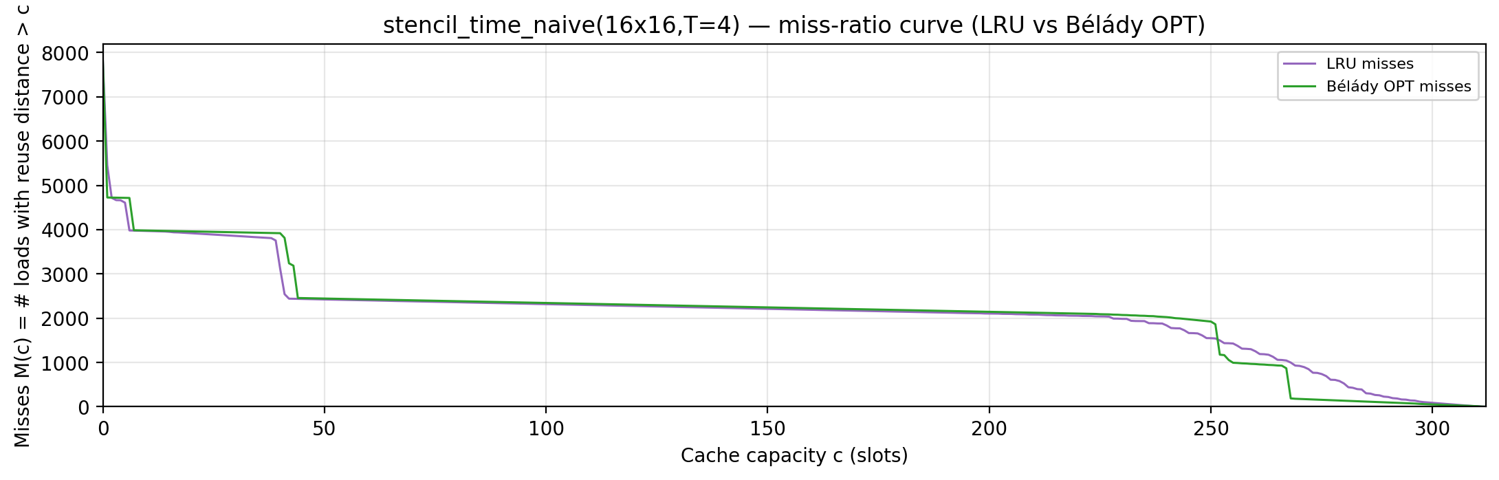
Per-tick TU LP floor — integrand of global_density: Σ_i ρ_{(i)} · √i over currently-live vars, ranked by density; the area equals global_density.

Per-tick splitting LP floor — integrand of local_density: Σ_i ρ_{(i)} · √i over the currently-active per-burst virtual intervals; the area equals the geometric portion of local_density.

Per-tick polymatroid LP floor — integrand of polymatroid_lb: Σ_v reads_v · ⌈√d_v⌉ / lifespan(v) over live vars, where d_v is each variable’s LP-implied static depth (gemini/polymatroid-relaxation.md). The area equals the geometric portion of polymatroid_lb.
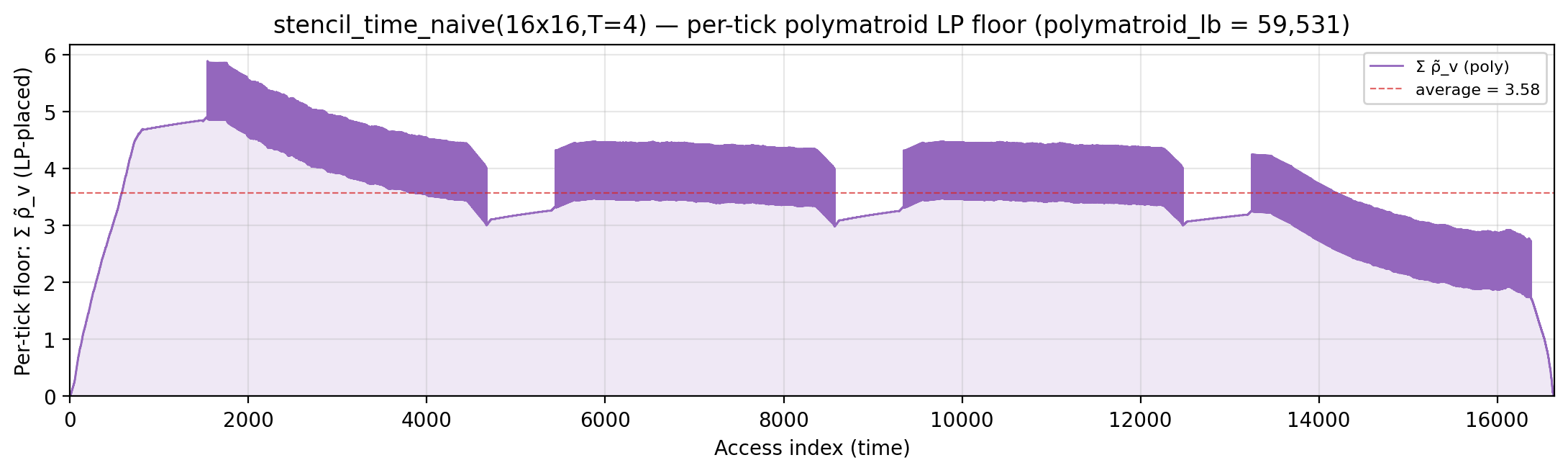
Rolling spatial intensity — heartbeat plot of ops / Σ ⌈√d⌉ over a sliding window.
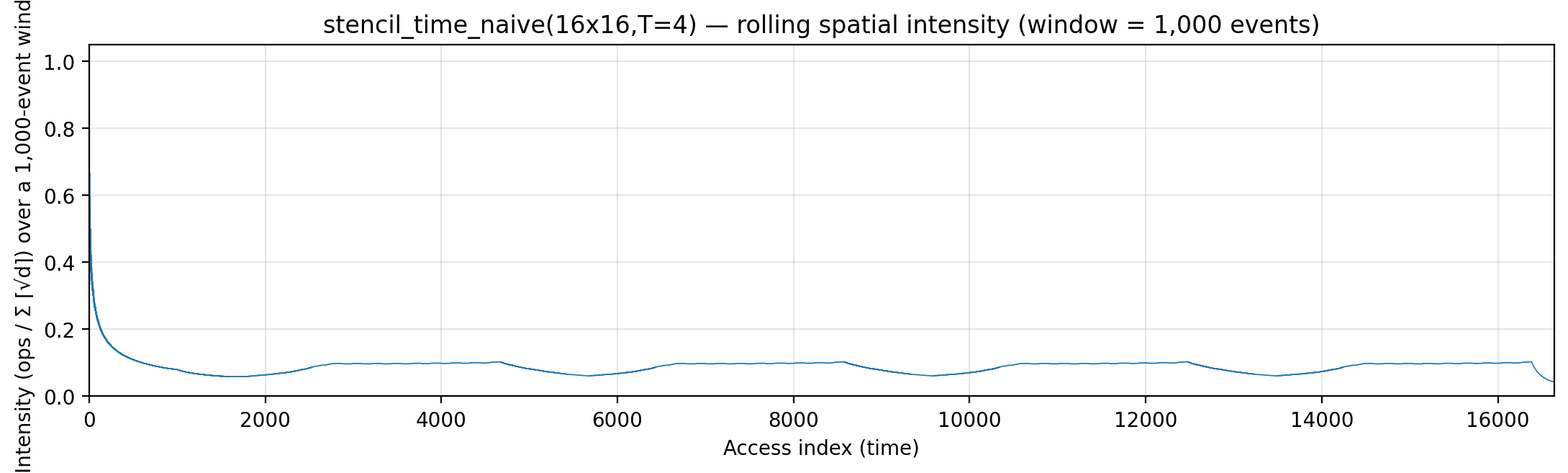
Cumulative compute vs fetch cost — slope = instantaneous spatial arithmetic intensity.
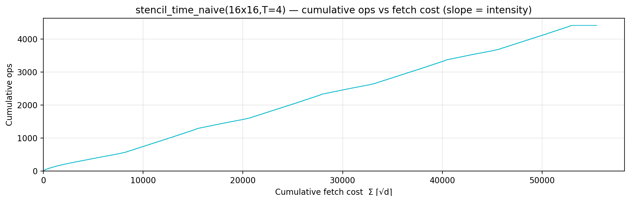
Gravity well — per-load fetch-cost ⌈√d⌉ scatter.
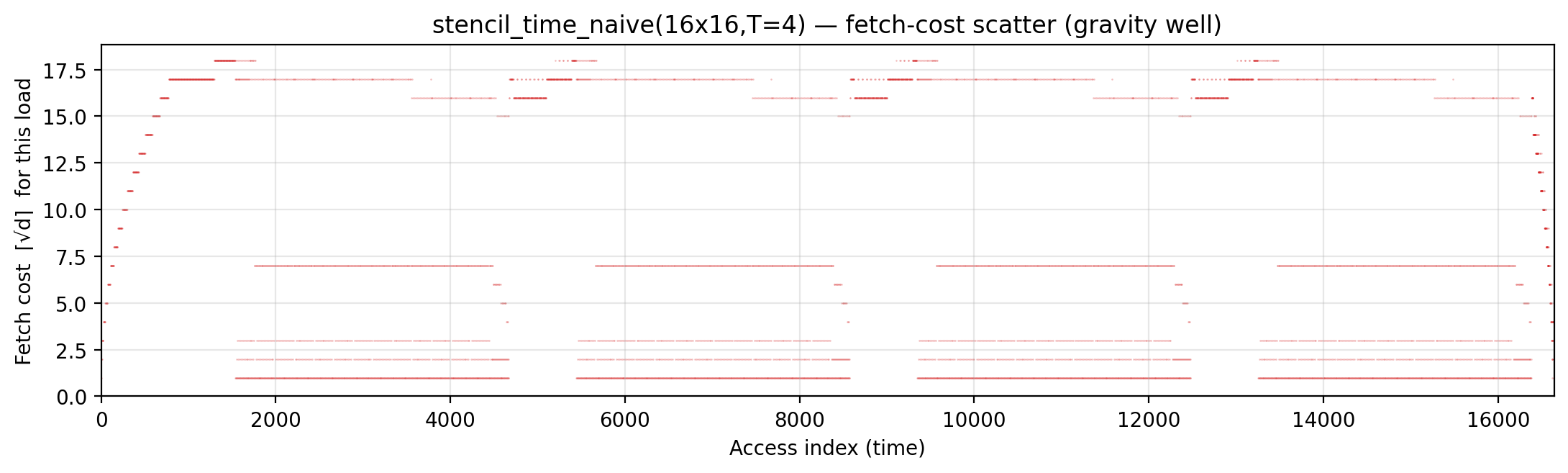
Spatial locality CDF — compute-fulfillment as a function of radius.
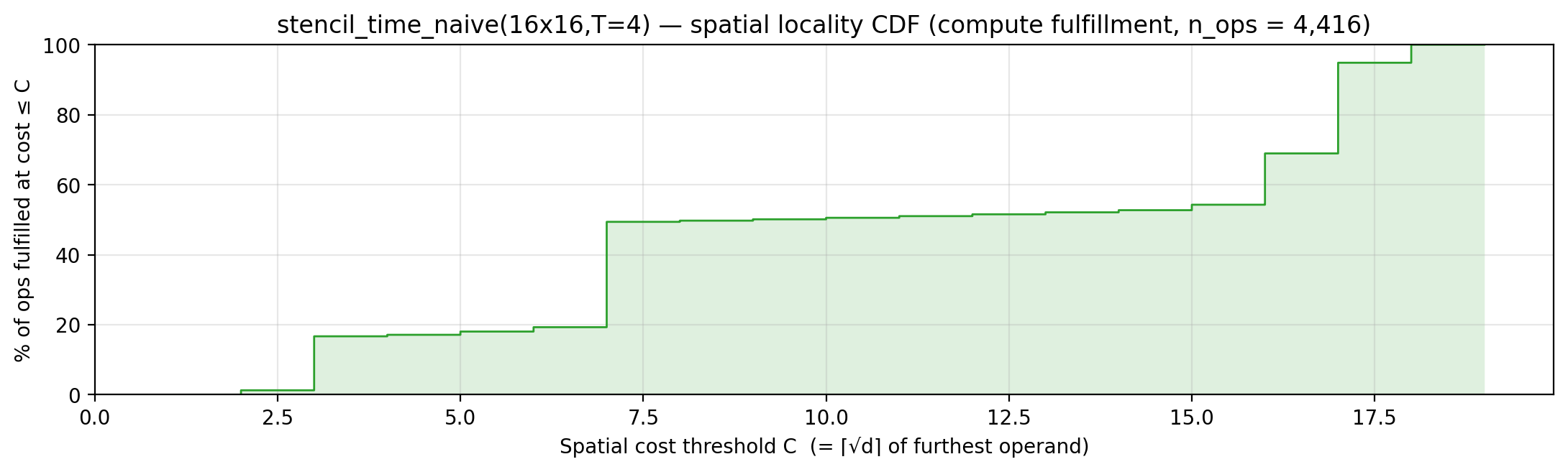
Working-set size over a τ = 273-event window (max = 264).
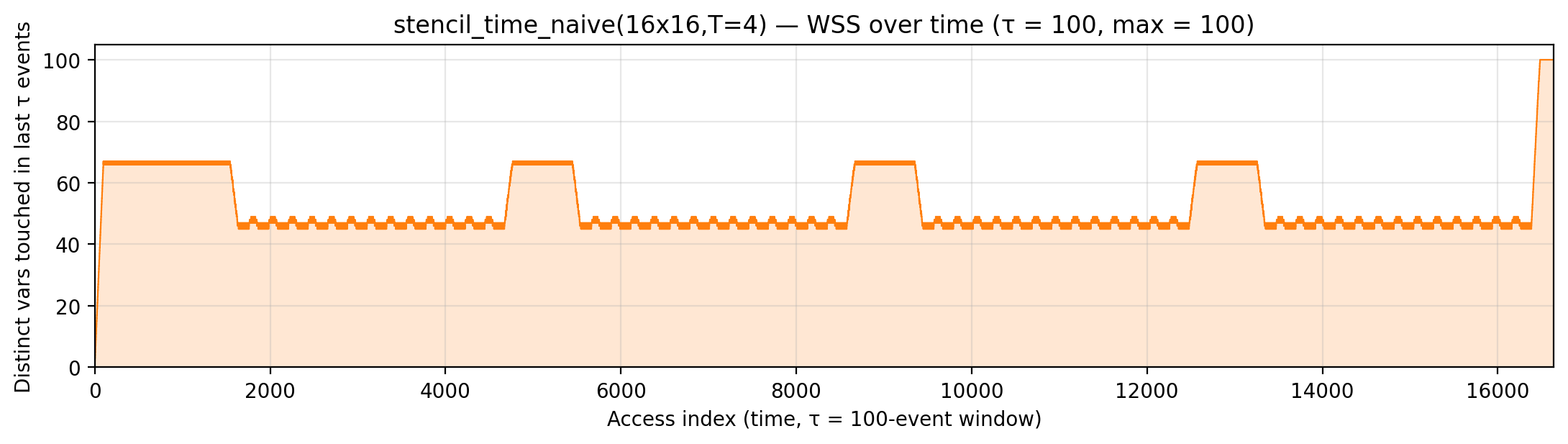
stencil_time_diamond (code)
n=16, T=4, block=4. Algorithm. Diamond tiling: per (bi,bj) block, load a halo-expanded region into a hot scratchpad and run all T steps locally before flushing.
Manual. Three stacked optimizations (gemini’s suggestion in
gemini/optimize-stencil-time-diamond.md):
- Lazy arg loading — only cells actually inside the current
block’s Manhattan-distance diamond (
dist_i + dist_j ≤ T) get touched, and only on their first visit. The naive version preloaded the full n² grid. - In-place time-stepping — the second
buf_nxtarray is dropped entirely. A sliding horizontal window of three scalar registersc_left / c_center / c_rightplus aprev_rowbuffer holds the stale neighbor values long enough to do an in-place write onbuf_cur. - Diamond pruning — each time step
tclips to the shrinking dependence conedist_i + dist_j ≤ T - 1 - t, so cells near the halo edge (whose values would be overwritten by halo contamination before they become needed) get skipped.
Layout:
c_left, c_center, c_right (addrs 1..3) — sliding L1 register ring;
prev_row (addrs 4..stride+3) — top-row buffer;
buf_cur (addrs stride+4..stride²+stride+3) — sole block workspace;
cur (addrs stride²+stride+4..) — global target.
Drops manual from 562,290 to 136,095 (−76%). Now beats
bytedmd_live (127,264 manual cost vs the 230,387 of the abstract
trace) — a rare win on an algorithm that was previously our
worst-ratio offender.
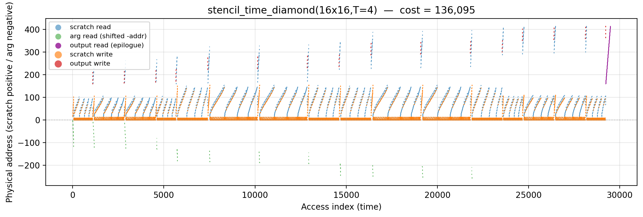
Working-set size over time (peak = 424).
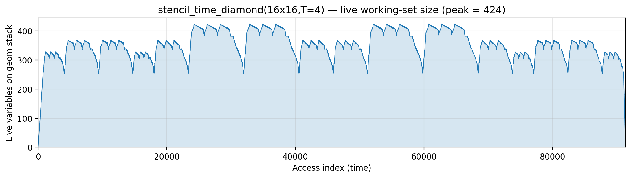
Reuse distance per load — LRU vs Bélády OPT (max LRU = 383; max OPT = 380).
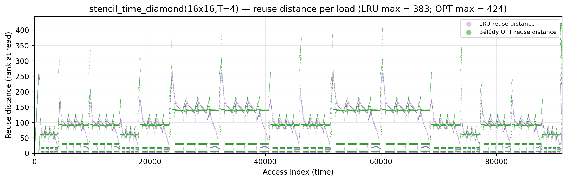
Miss-ratio curve — LRU vs Bélády OPT misses by cache capacity.
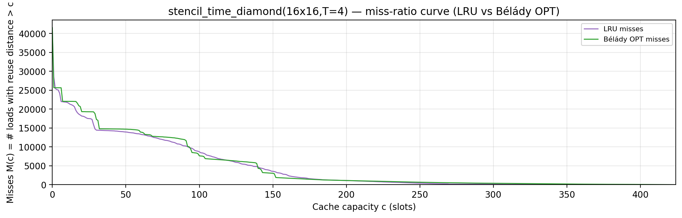
Per-tick TU LP floor — integrand of global_density: Σ_i ρ_{(i)} · √i over currently-live vars, ranked by density; the area equals global_density.

Per-tick splitting LP floor — integrand of local_density: Σ_i ρ_{(i)} · √i over the currently-active per-burst virtual intervals; the area equals the geometric portion of local_density.

Rolling spatial intensity — heartbeat plot of ops / Σ ⌈√d⌉ over a sliding window.
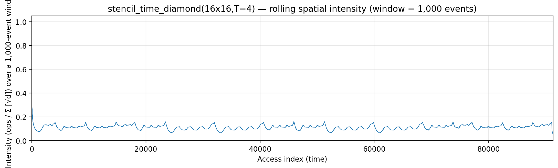
Cumulative compute vs fetch cost — slope = instantaneous spatial arithmetic intensity.
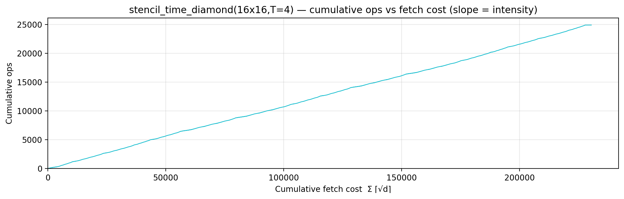
Gravity well — per-load fetch-cost ⌈√d⌉ scatter.
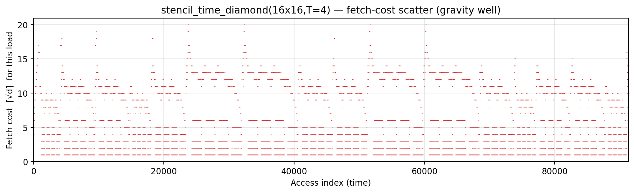
Spatial locality CDF — compute-fulfillment as a function of radius.
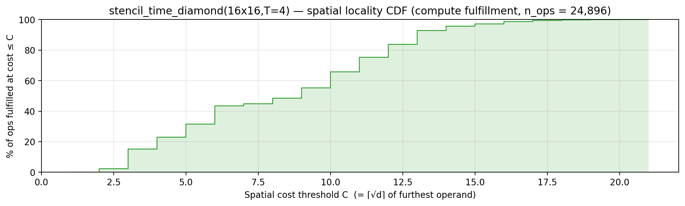
Working-set size over a τ = 145-event window (max = 145).
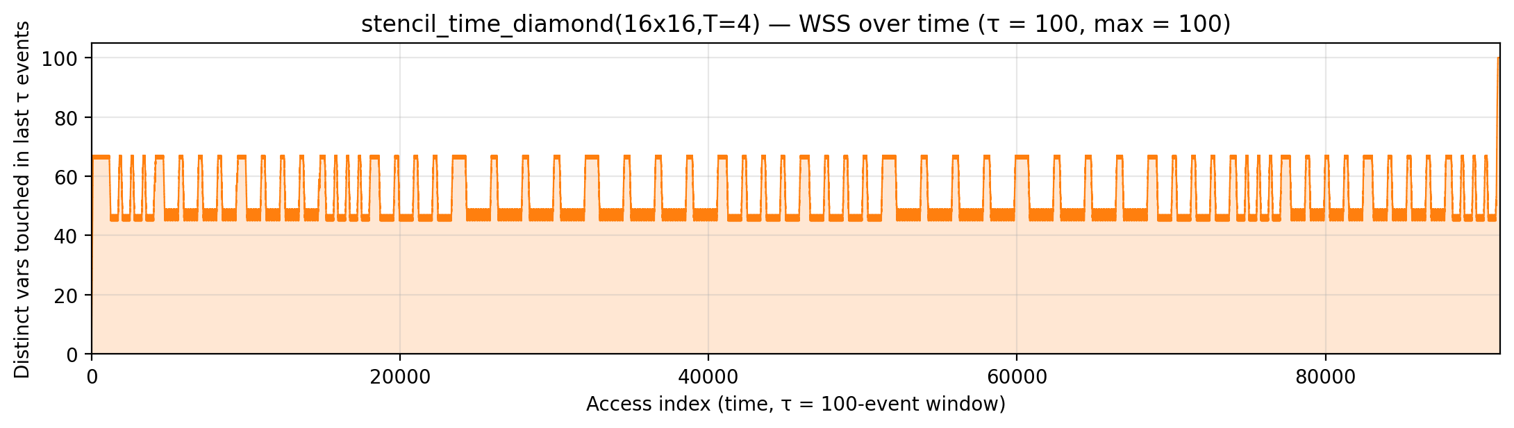
floyd_warshall_naive (code)
V=16. Algorithm. Standard 3-nested loop APSP: D[i][j] = min(D[i][j], D[i][k] + D[k][j]) with branch-free stand-ins.
Manual. Same A[i][j] -= A[i][k] · A[k][j] inner body as
lu_no_pivot — apply the same hoisting recipe:
c_A (addr 1) — hot scalar pinning D[i][k] across j-sweep
c_C (addrs 2..V+1) — row buffer caching D[k][0..V-1]
D (addrs V+2..) — scratch graph
Lazy arg reads at k=0 replace the V² preload. Drops manual from
142,800 to 76,339 (−47%), now within 2 % of global_density
(74,923).
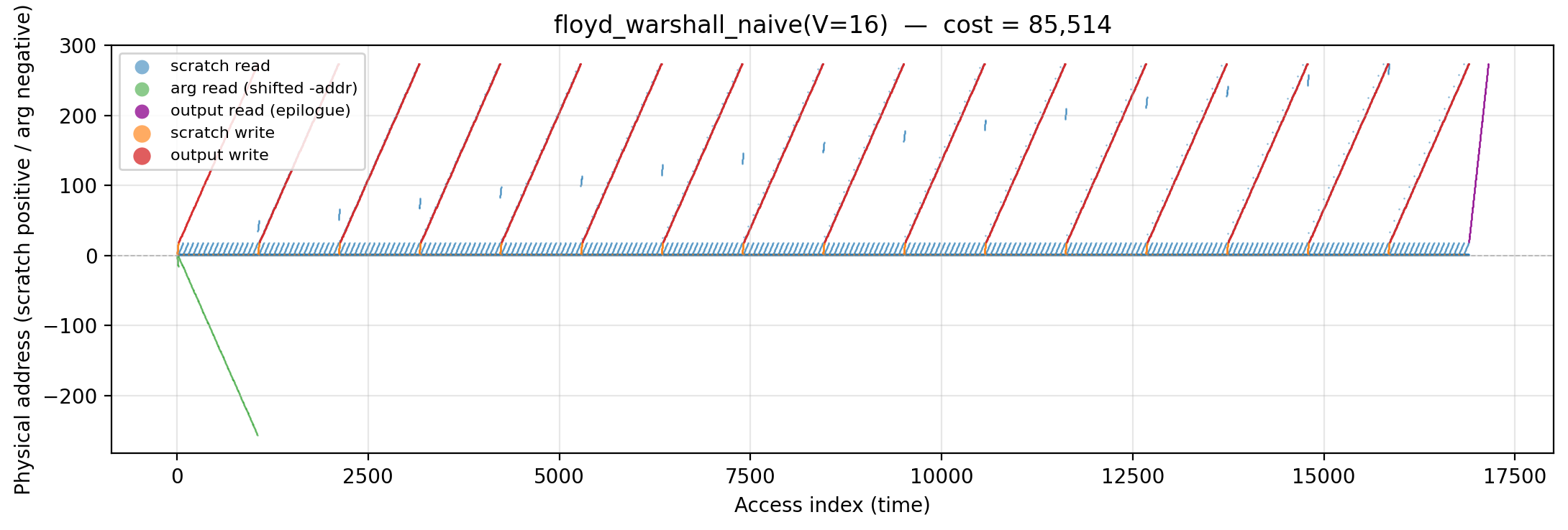
Working-set size over time (peak = 257).
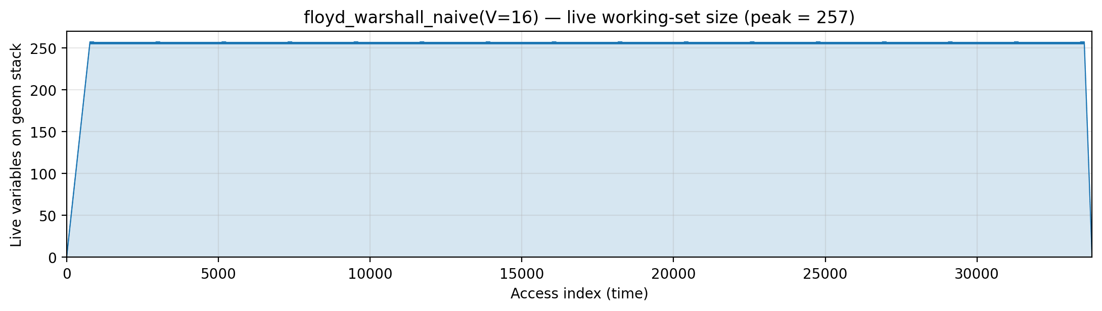
Reuse distance per load — LRU vs Bélády OPT (max LRU = 256; max OPT = 256).
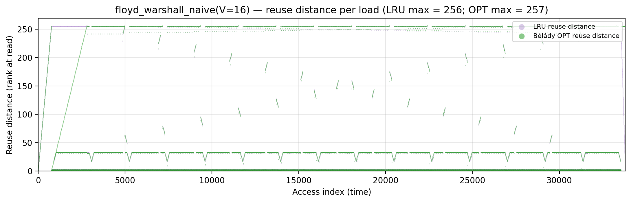
Miss-ratio curve — LRU vs Bélády OPT misses by cache capacity.
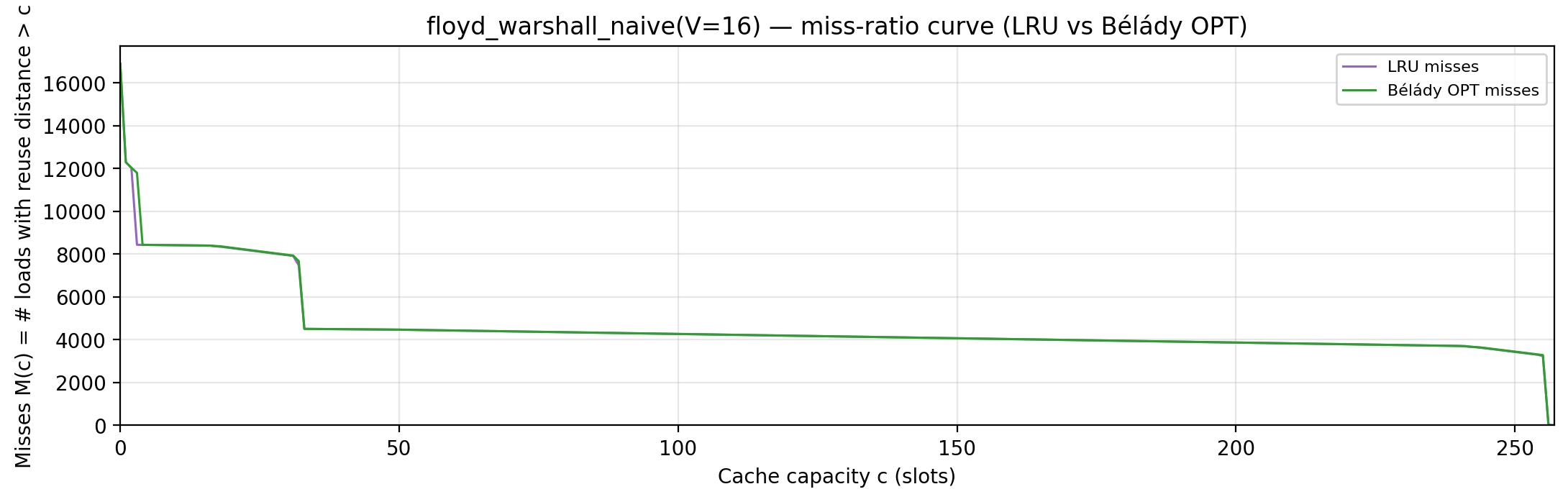
Per-tick TU LP floor — integrand of global_density: Σ_i ρ_{(i)} · √i over currently-live vars, ranked by density; the area equals global_density.
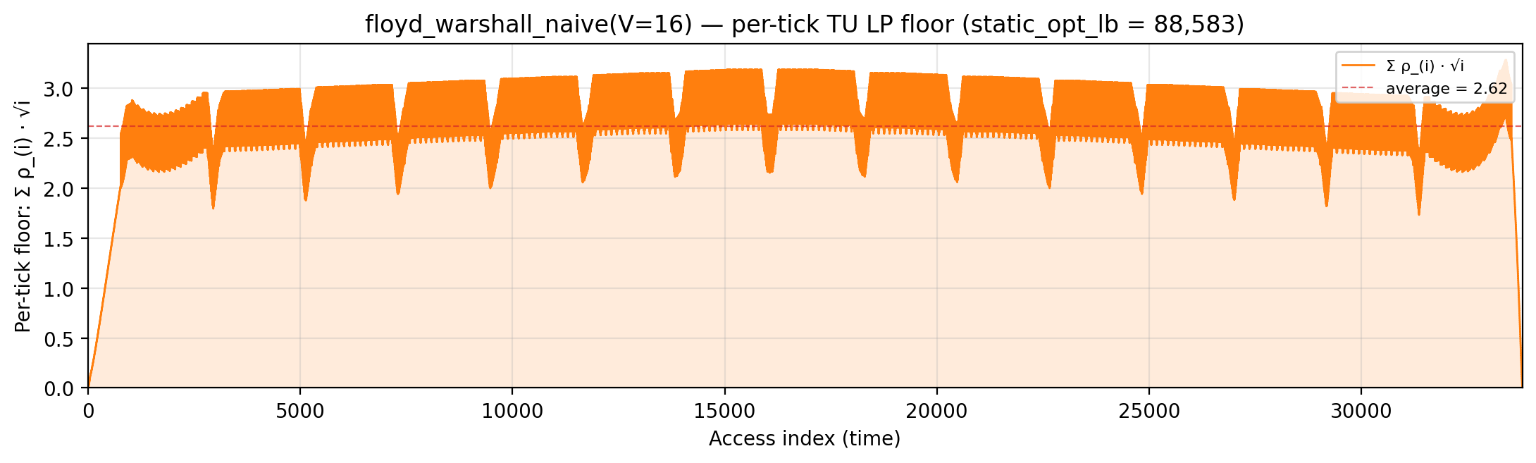
Per-tick splitting LP floor — integrand of local_density: Σ_i ρ_{(i)} · √i over the currently-active per-burst virtual intervals; the area equals the geometric portion of local_density.
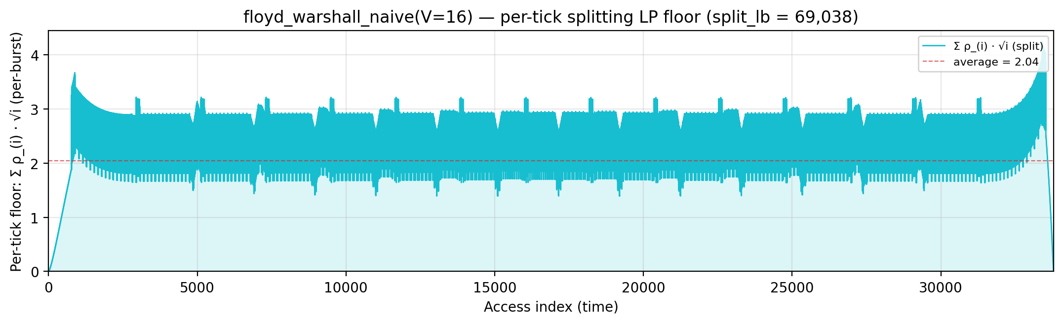
Per-tick polymatroid LP floor — integrand of polymatroid_lb: Σ_v reads_v · ⌈√d_v⌉ / lifespan(v) over live vars, where d_v is each variable’s LP-implied static depth (gemini/polymatroid-relaxation.md). The area equals the geometric portion of polymatroid_lb.
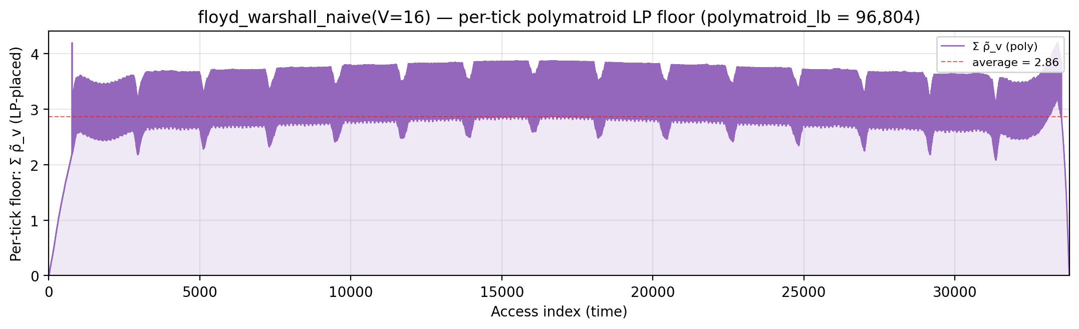
Rolling spatial intensity — heartbeat plot of ops / Σ ⌈√d⌉ over a sliding window.
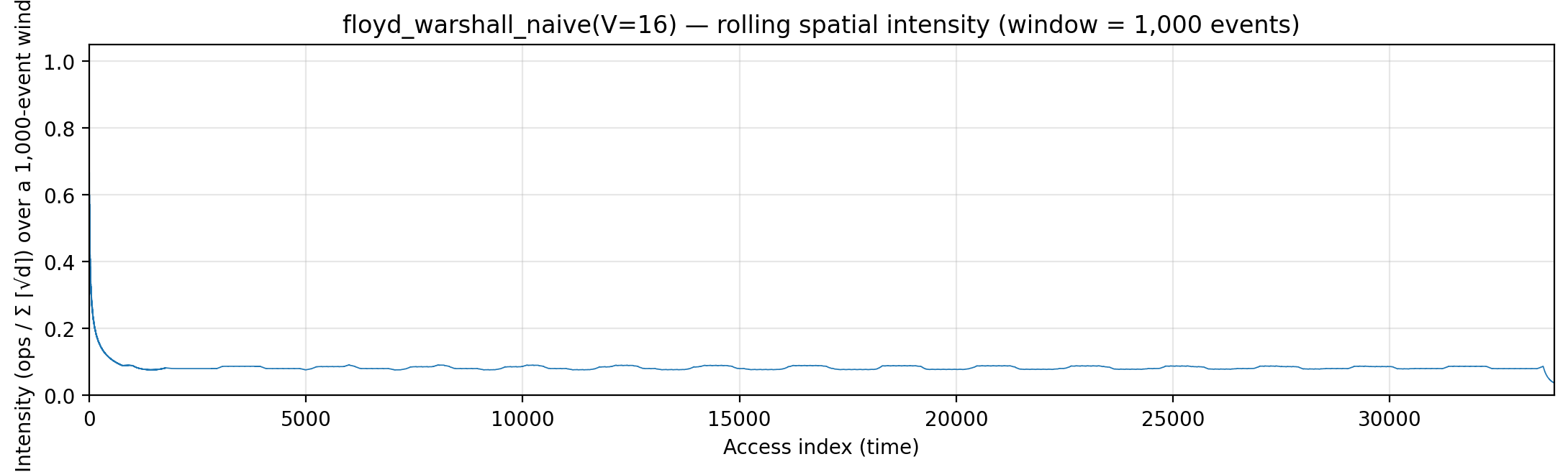
Cumulative compute vs fetch cost — slope = instantaneous spatial arithmetic intensity.
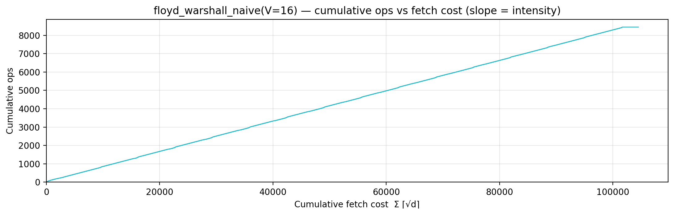
Gravity well — per-load fetch-cost ⌈√d⌉ scatter.
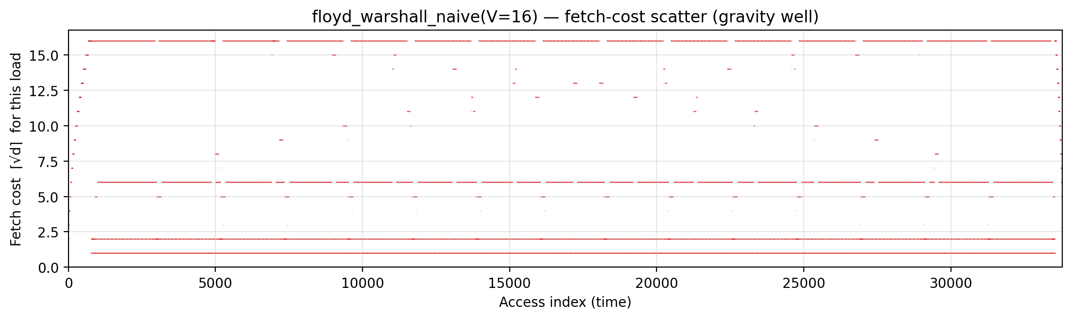
Spatial locality CDF — compute-fulfillment as a function of radius.
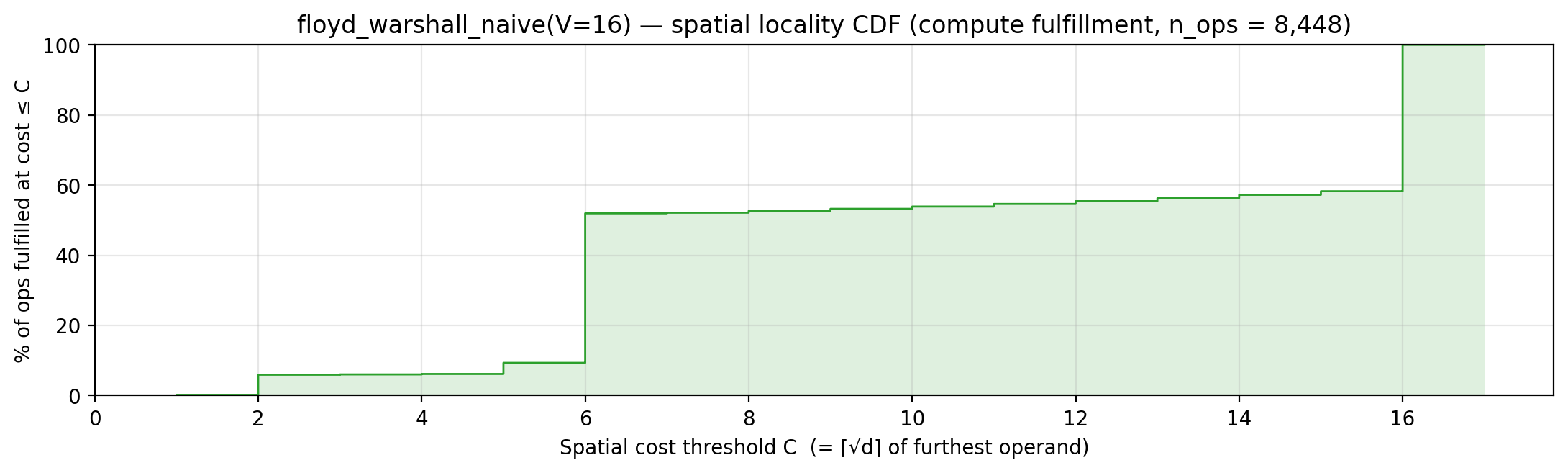
Working-set size over a τ = 256-event window (max = 256).
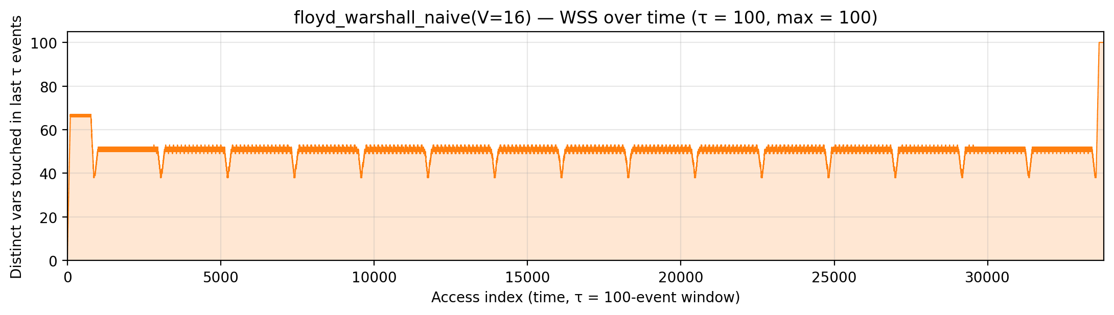
floyd_warshall_recursive (code)
V=16. Algorithm. Kleene’s cache-oblivious APSP: 8 recursive quadrant calls per level.
Manual. Three stacked optimizations (gemini/optimize-floyd-warshall-recursive.md):
- L1 scratchpads at stack bottom —
cache_T(target block) andcache_D(diagonal block), each 2×2, pinned at addresses 1..8. The O(V³) inner loops run entirely inside those 8 cells. - Dirty-tracking — the target block is only flushed back to
Dwhen a new block is loaded and the previous one was written to. - Frequency-ordered layout — a dry run counts cache misses per
leaf block;
Dis then physically laid out with the highest-miss blocks at the lowest addresses via aD_addr(r, c)remap.
Drops manual from 142,288 to 57,920 (−59%), now only 22% above
bytedmd_live (47,495) vs the old 3.00× — one of the biggest
single-algorithm wins in the grid.
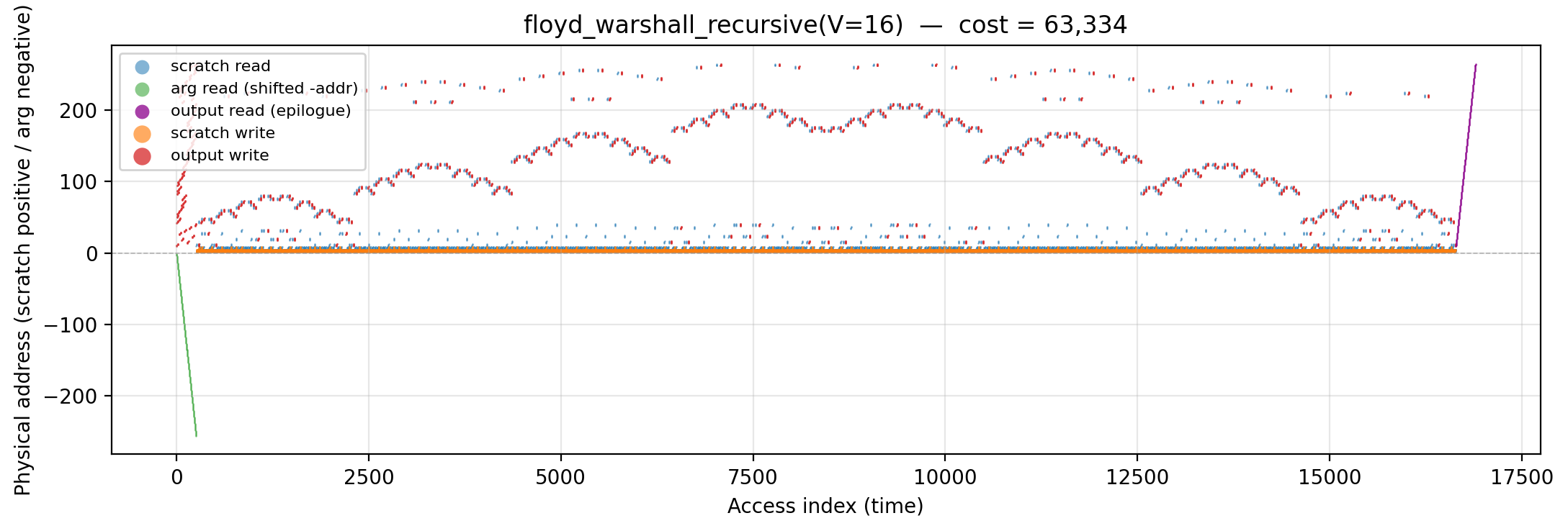
Working-set size over time (peak = 257).
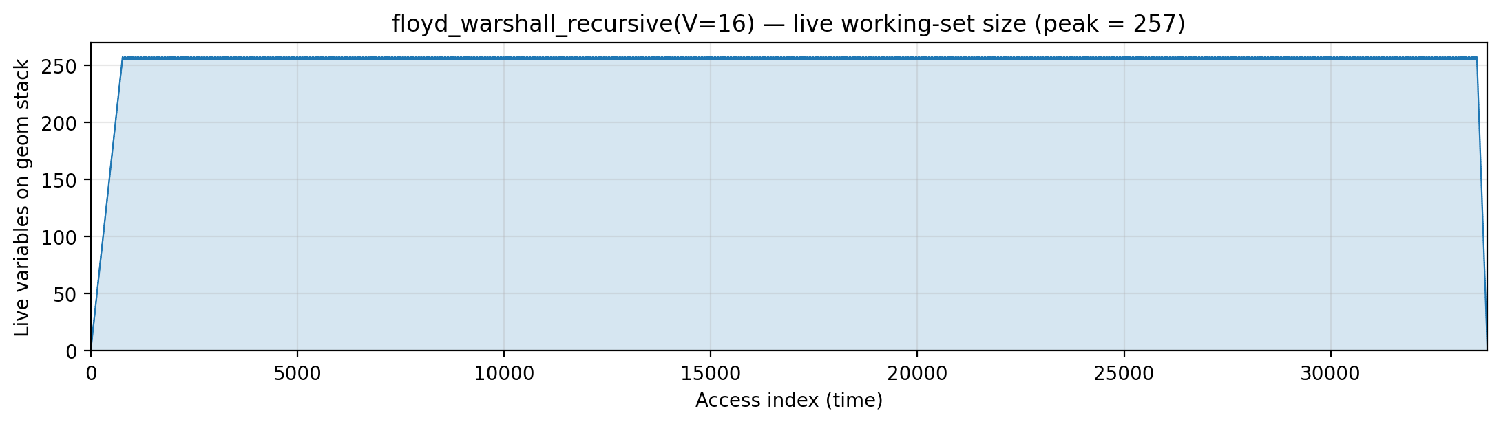
Reuse distance per load — LRU vs Bélády OPT (max LRU = 256; max OPT = 256).
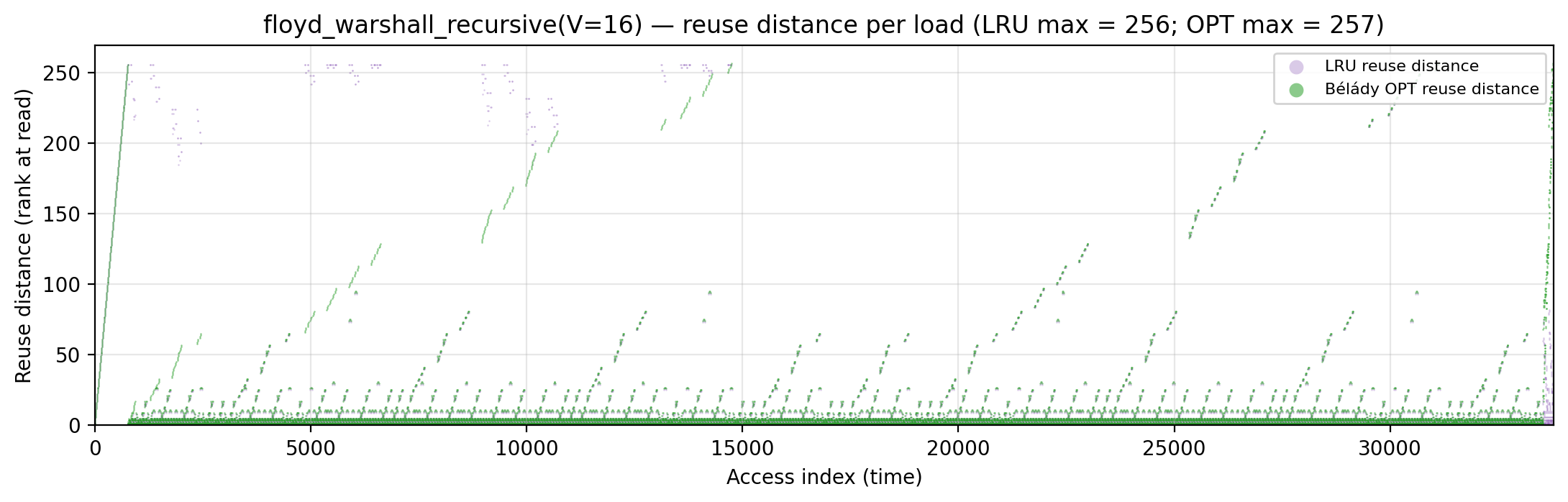
Miss-ratio curve — LRU vs Bélády OPT misses by cache capacity.
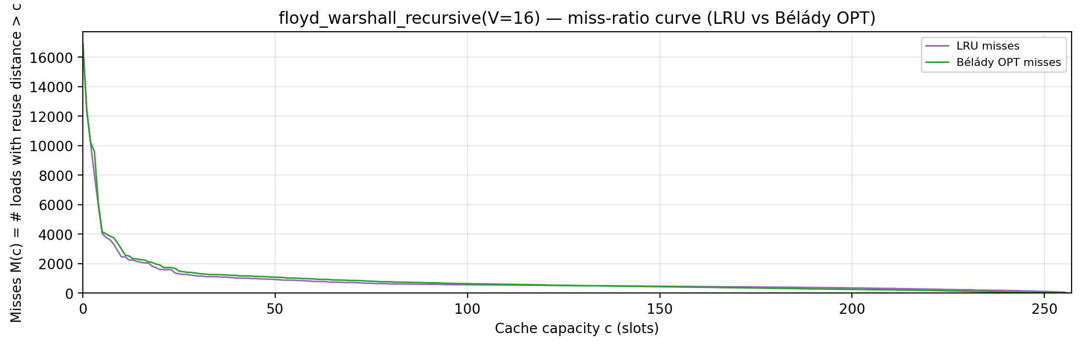
Per-tick TU LP floor — integrand of global_density: Σ_i ρ_{(i)} · √i over currently-live vars, ranked by density; the area equals global_density.
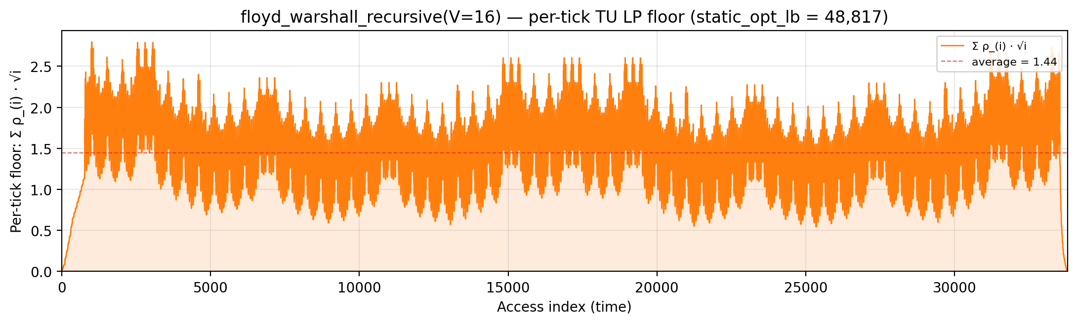
Per-tick splitting LP floor — integrand of local_density: Σ_i ρ_{(i)} · √i over the currently-active per-burst virtual intervals; the area equals the geometric portion of local_density.
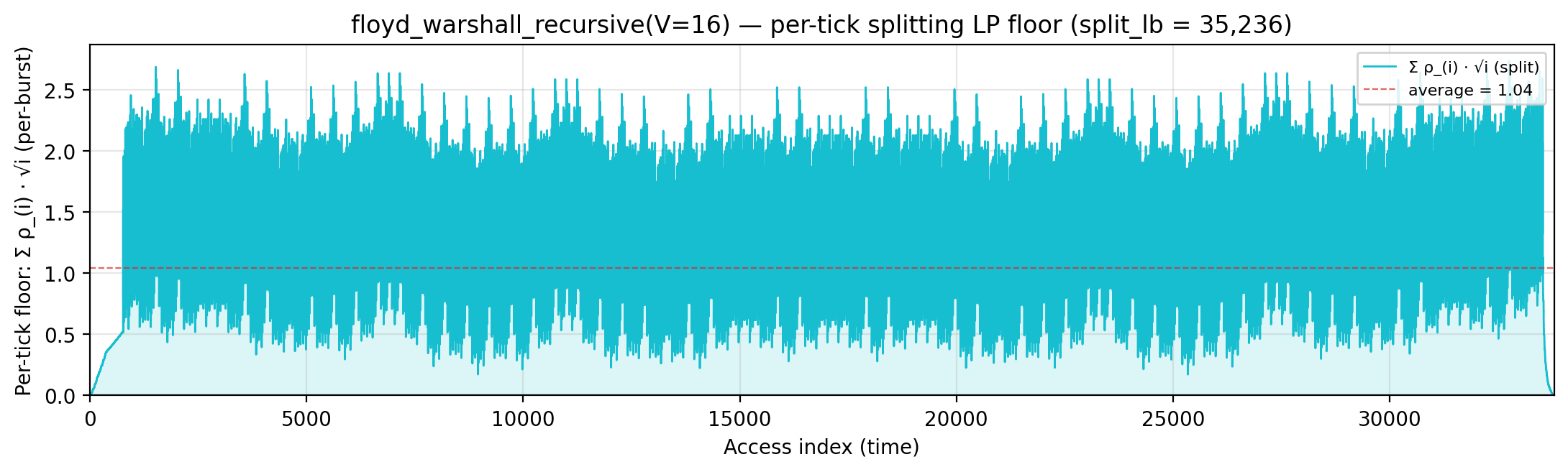
Per-tick polymatroid LP floor — integrand of polymatroid_lb: Σ_v reads_v · ⌈√d_v⌉ / lifespan(v) over live vars, where d_v is each variable’s LP-implied static depth (gemini/polymatroid-relaxation.md). The area equals the geometric portion of polymatroid_lb.
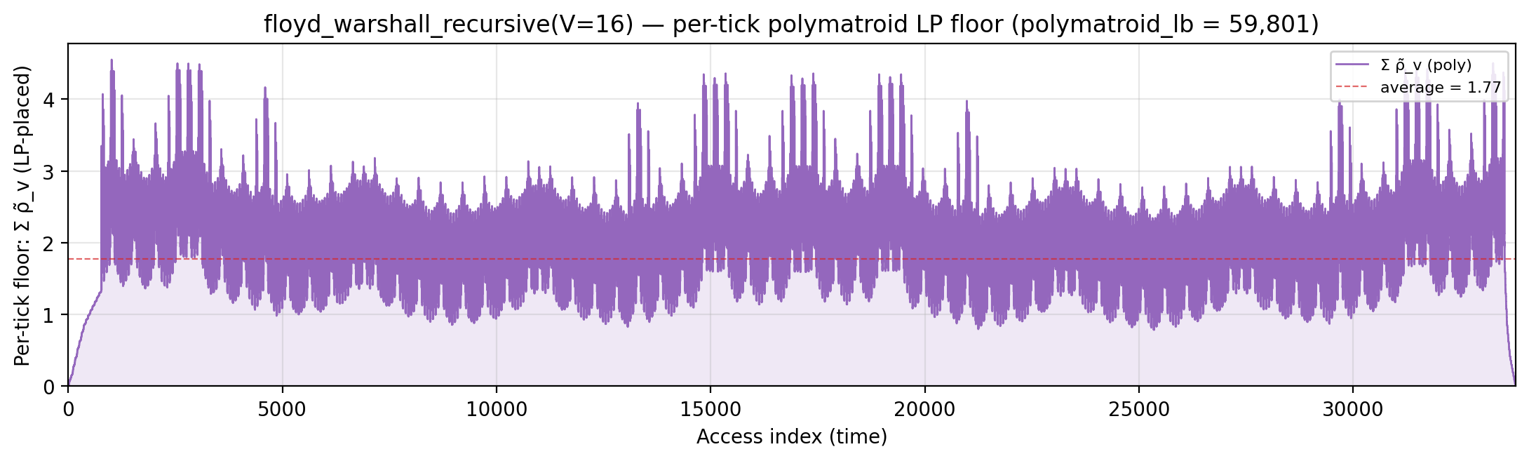
Rolling spatial intensity — heartbeat plot of ops / Σ ⌈√d⌉ over a sliding window.
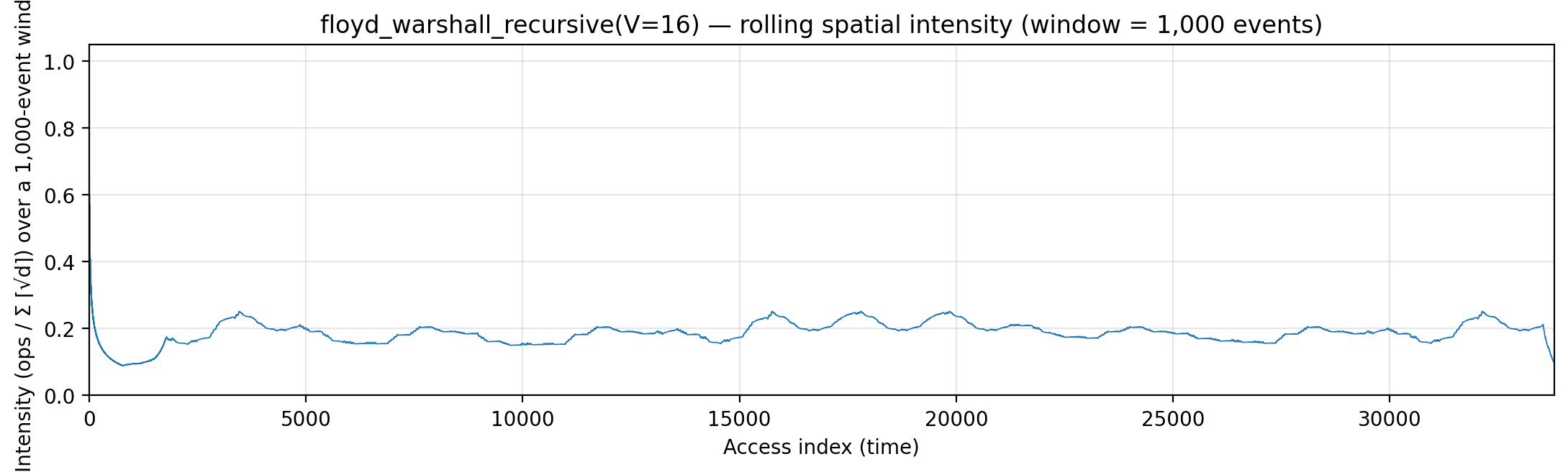
Cumulative compute vs fetch cost — slope = instantaneous spatial arithmetic intensity.
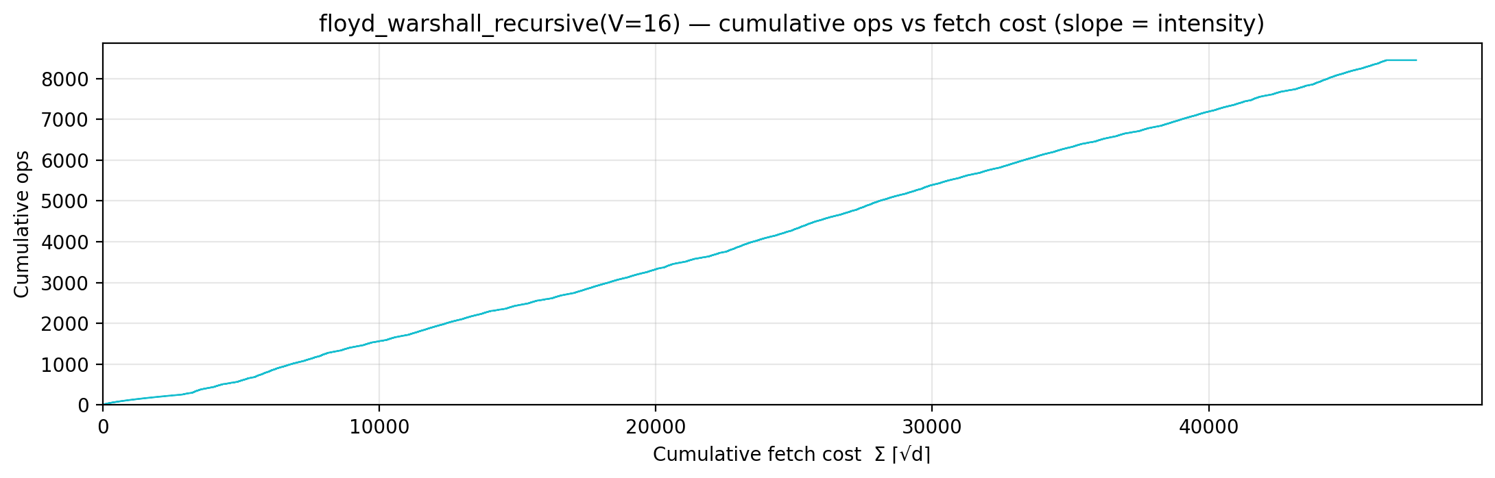
Gravity well — per-load fetch-cost ⌈√d⌉ scatter.
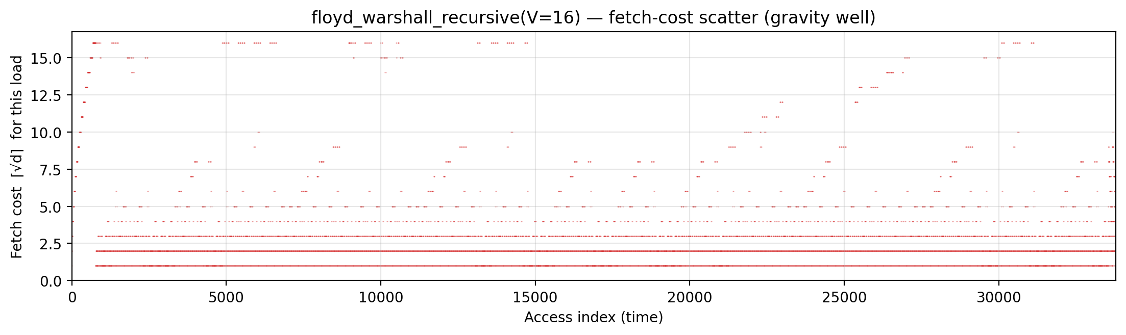
Spatial locality CDF — compute-fulfillment as a function of radius.
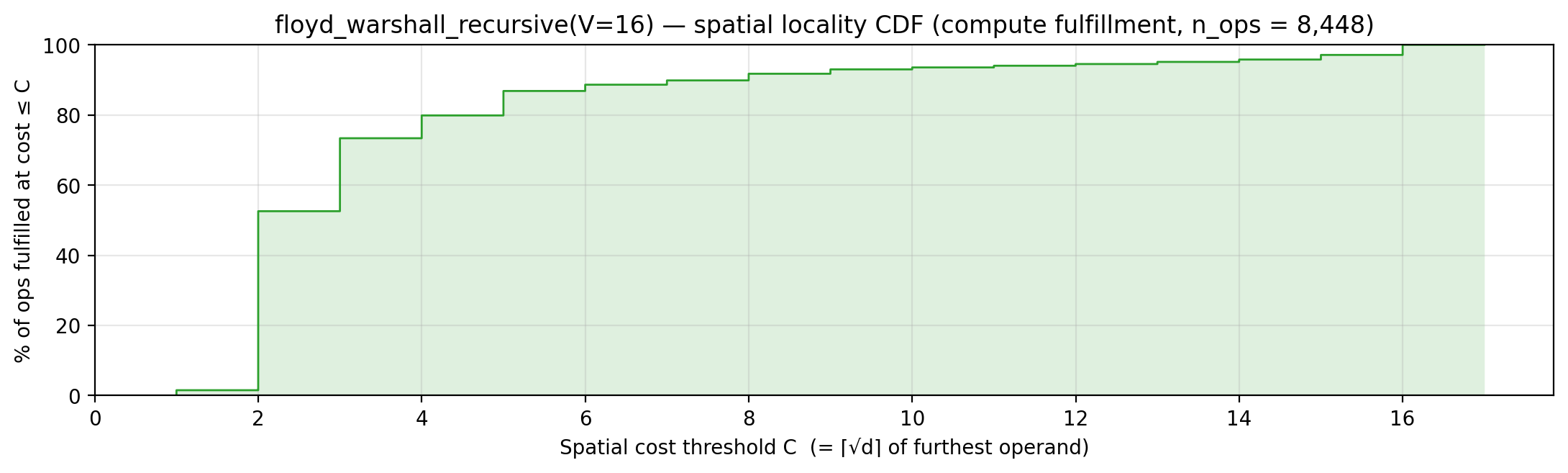
Working-set size over a τ = 32-event window (max = 32).
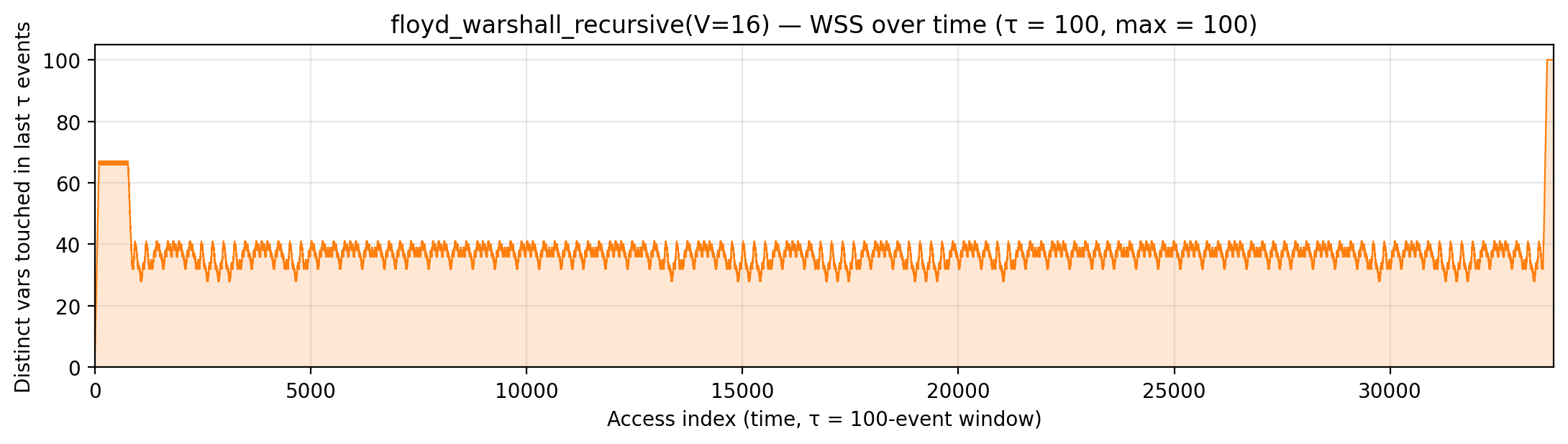
layernorm_unfused (code)
N=256. Algorithm. Three-pass LayerNorm: mean → variance → normalize. Each pass re-reads x from bulk.
Manual. x on arg stack; s/v/mean/inv_std scalars on scratch addrs 1-4 for hot accumulation. Output y on scratch.
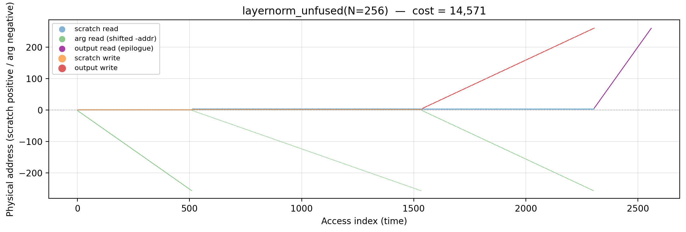
Working-set size over time (peak = 260).
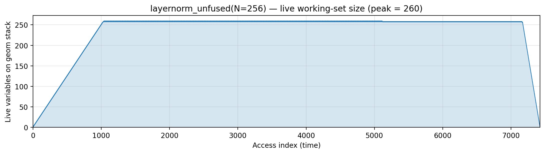
Reuse distance per load — LRU vs Bélády OPT (max LRU = 258; max OPT = 257).
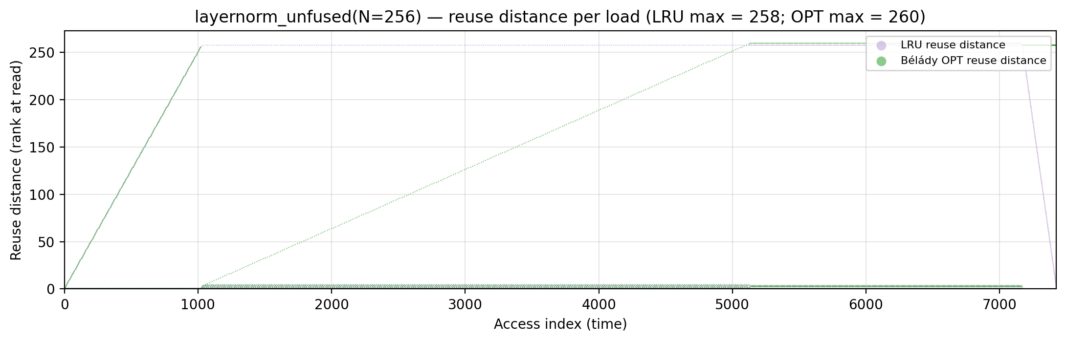
Miss-ratio curve — LRU vs Bélády OPT misses by cache capacity.
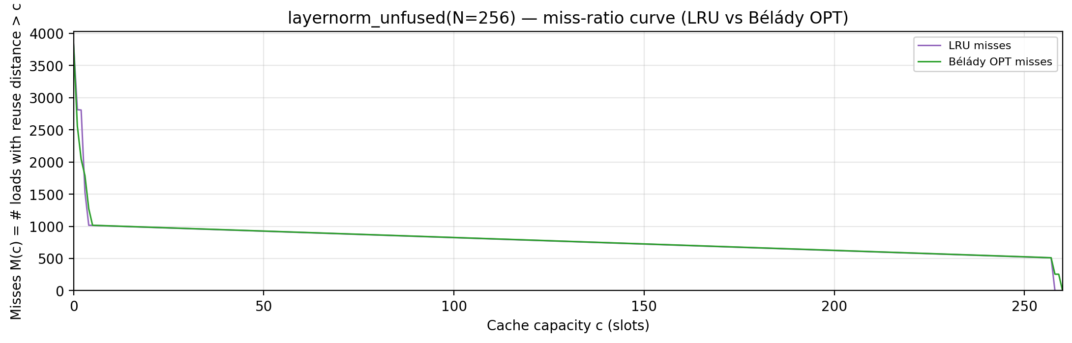
Per-tick TU LP floor — integrand of global_density: Σ_i ρ_{(i)} · √i over currently-live vars, ranked by density; the area equals global_density.
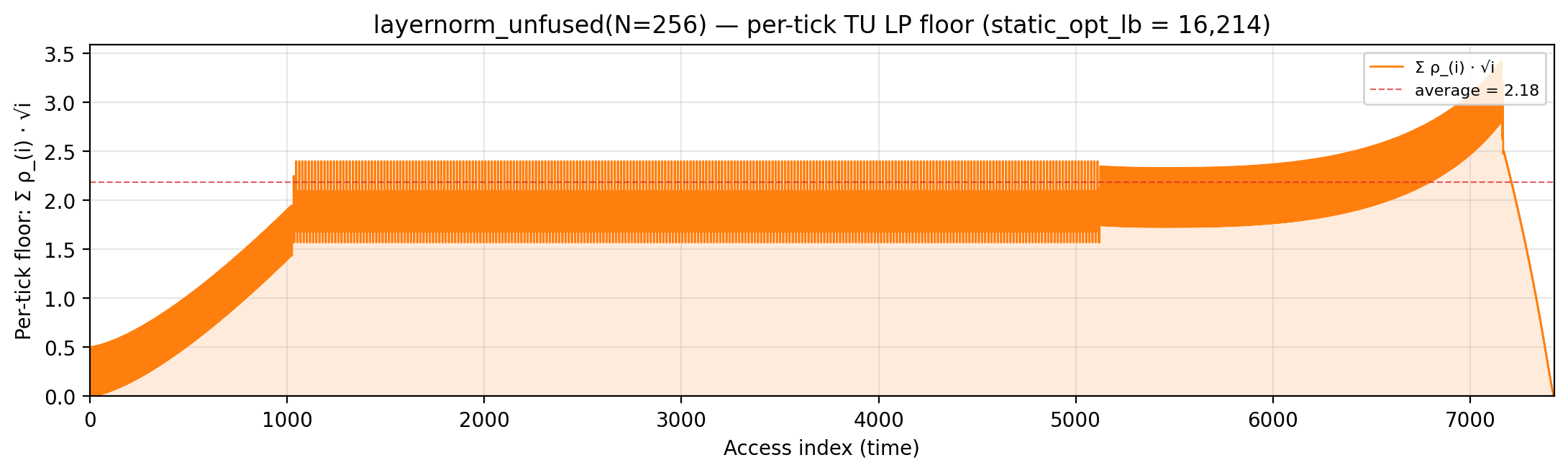
Per-tick splitting LP floor — integrand of local_density: Σ_i ρ_{(i)} · √i over the currently-active per-burst virtual intervals; the area equals the geometric portion of local_density.
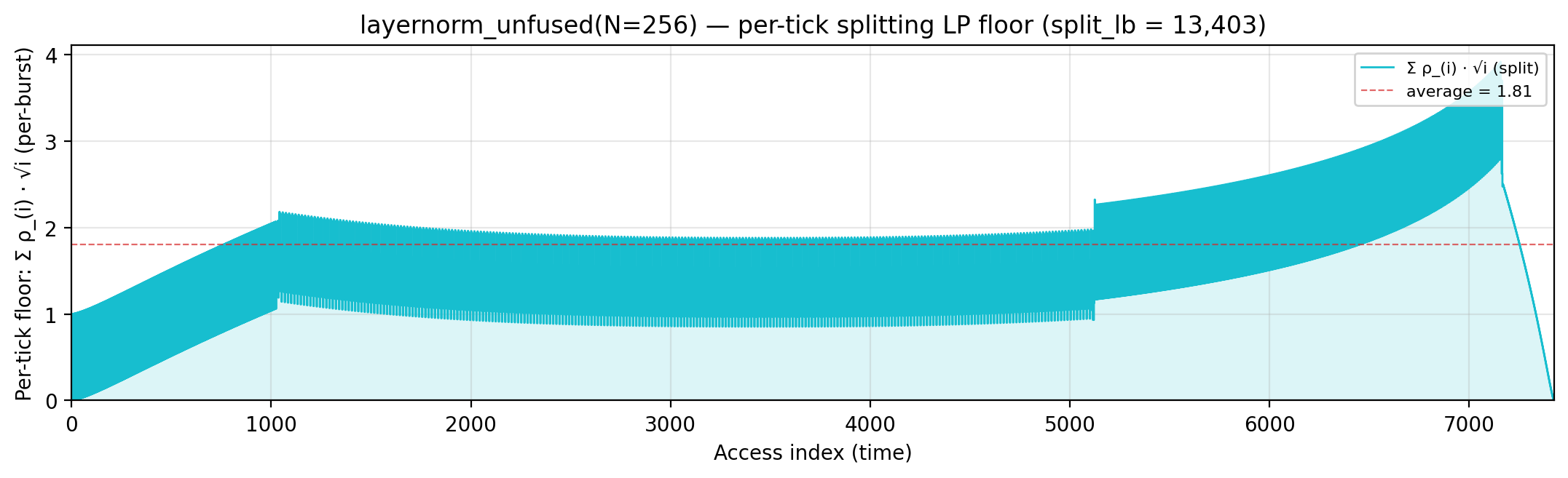
Per-tick polymatroid LP floor — integrand of polymatroid_lb: Σ_v reads_v · ⌈√d_v⌉ / lifespan(v) over live vars, where d_v is each variable’s LP-implied static depth (gemini/polymatroid-relaxation.md). The area equals the geometric portion of polymatroid_lb.
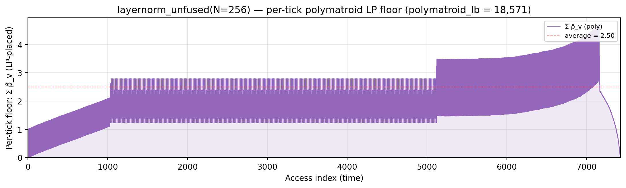
Rolling spatial intensity — heartbeat plot of ops / Σ ⌈√d⌉ over a sliding window.
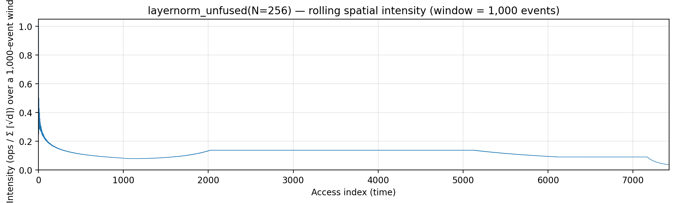
Cumulative compute vs fetch cost — slope = instantaneous spatial arithmetic intensity.
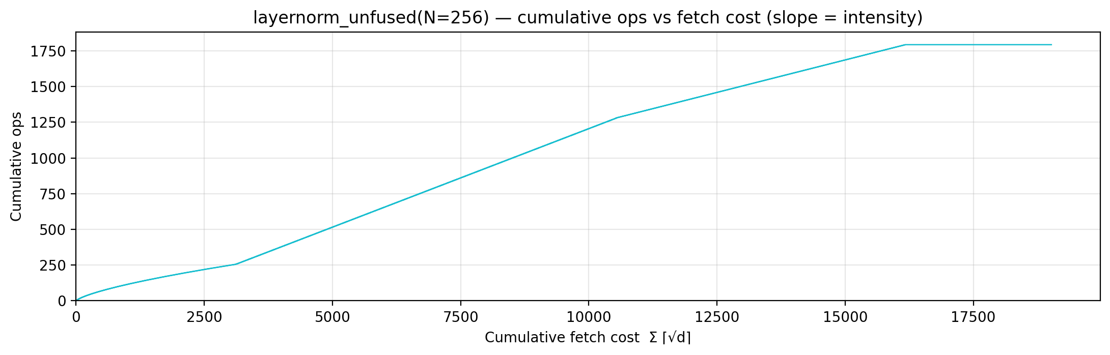
Gravity well — per-load fetch-cost ⌈√d⌉ scatter.
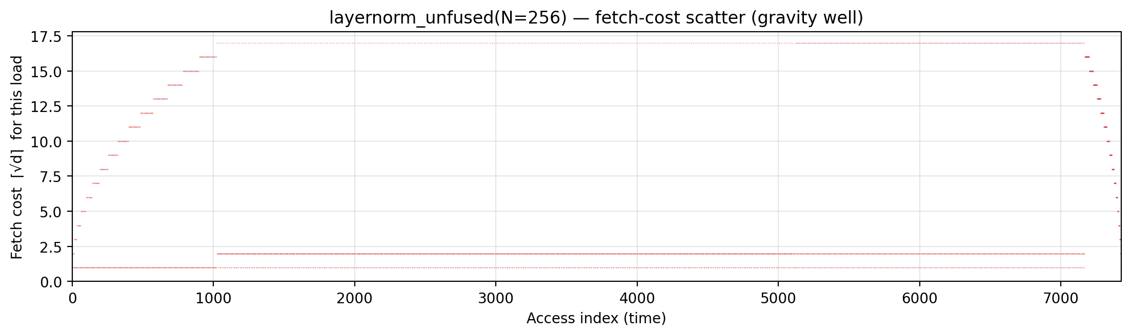
Spatial locality CDF — compute-fulfillment as a function of radius.
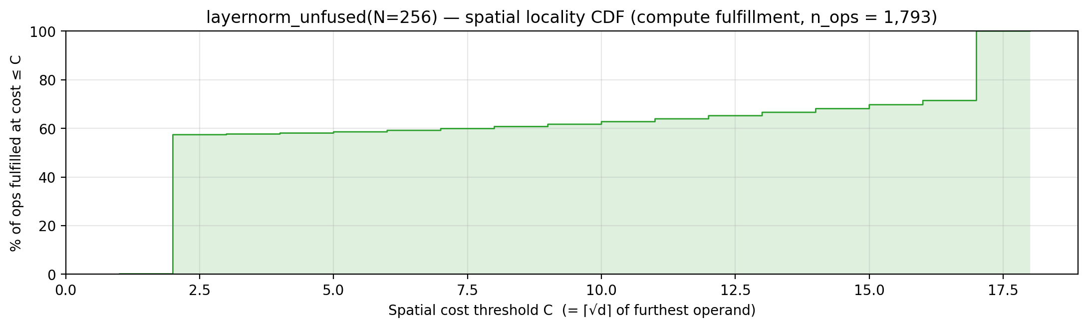
Working-set size over a τ = 258-event window (max = 257).
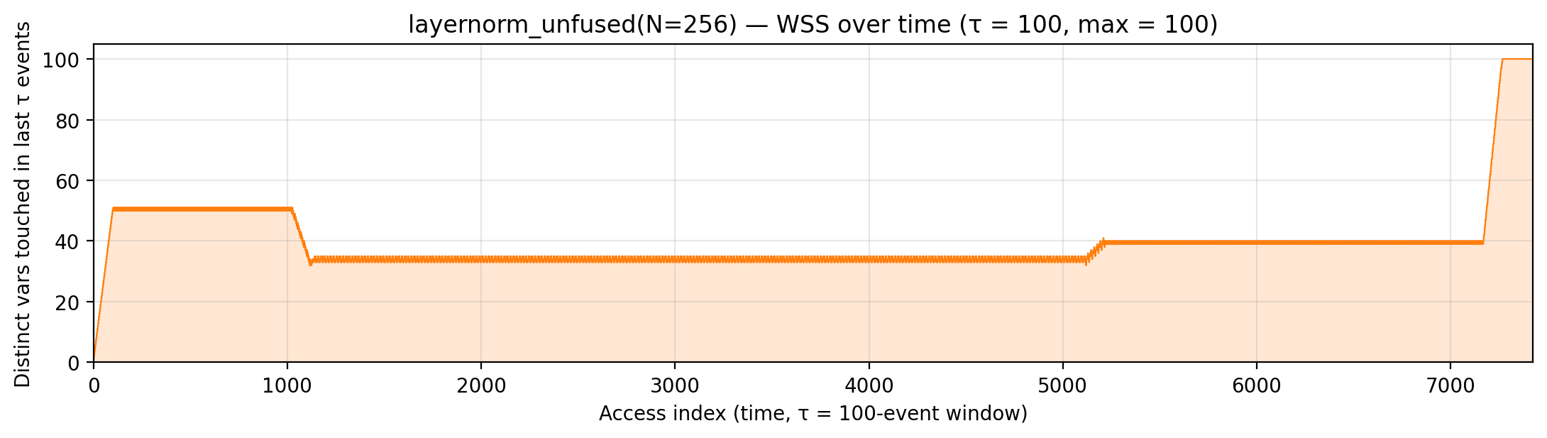
layernorm_fused (code)
N=256. Algorithm. Welford’s online mean+var in one pass, plus a second pass to normalize. The running accumulators stay in hot registers across all N updates.
Manual. Fewer address-space traversals — mu and m2 are read and written O(N) times but stay at depth 1-2 throughout.
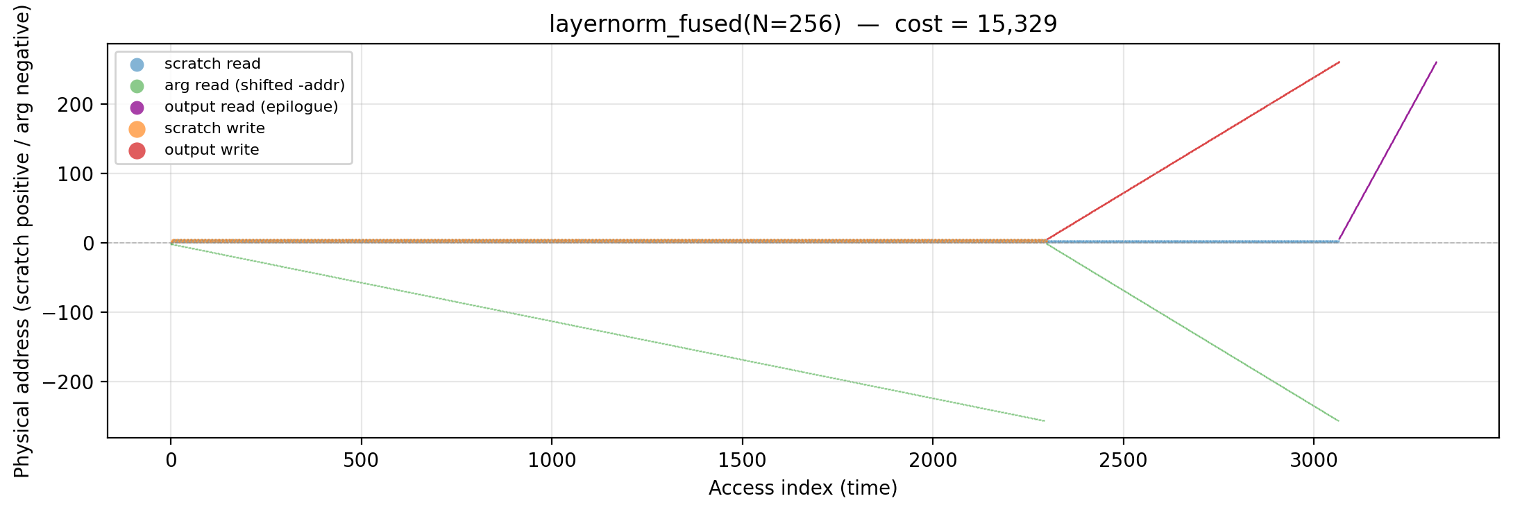
Working-set size over time (peak = 260).
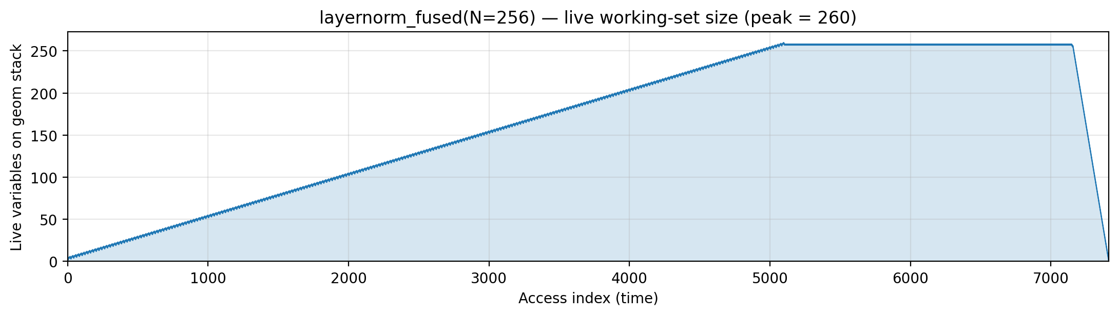
Reuse distance per load — LRU vs Bélády OPT (max LRU = 258; max OPT = 258).
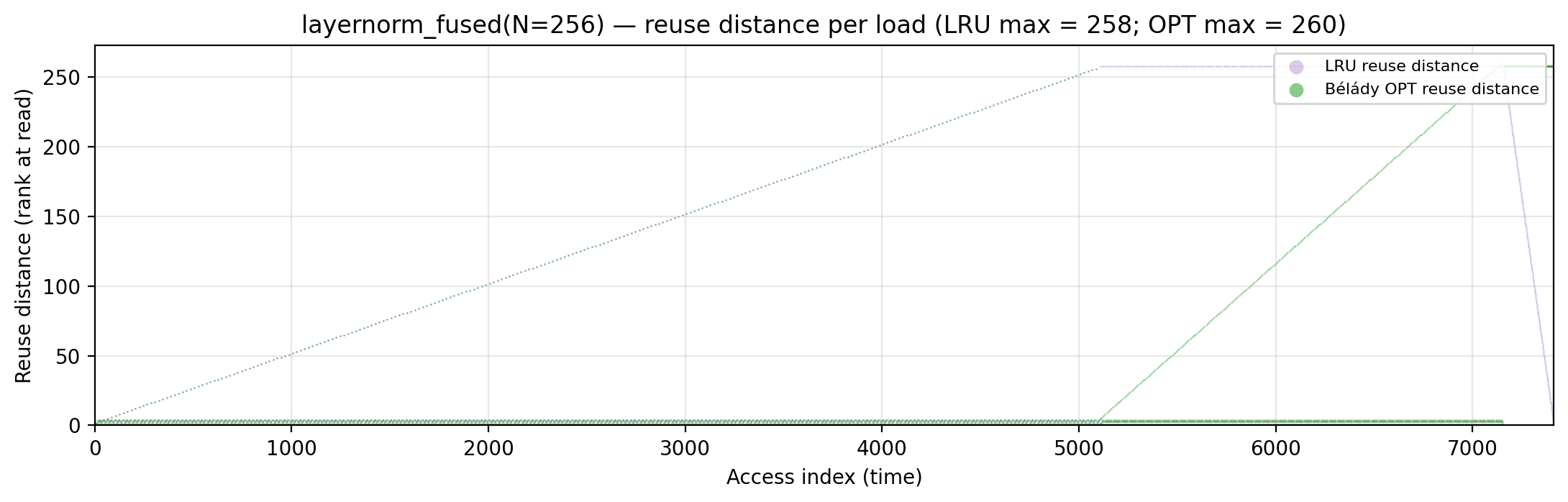
Miss-ratio curve — LRU vs Bélády OPT misses by cache capacity.
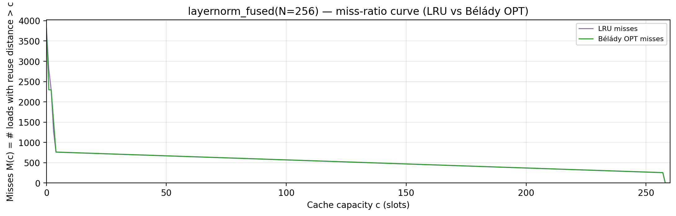
Per-tick TU LP floor — integrand of global_density: Σ_i ρ_{(i)} · √i over currently-live vars, ranked by density; the area equals global_density.
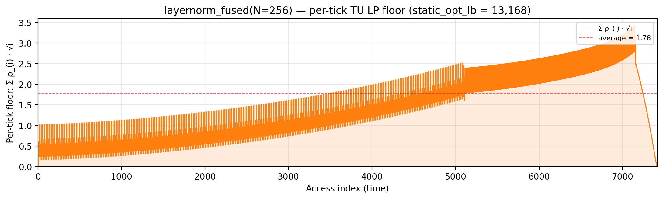
Per-tick splitting LP floor — integrand of local_density: Σ_i ρ_{(i)} · √i over the currently-active per-burst virtual intervals; the area equals the geometric portion of local_density.
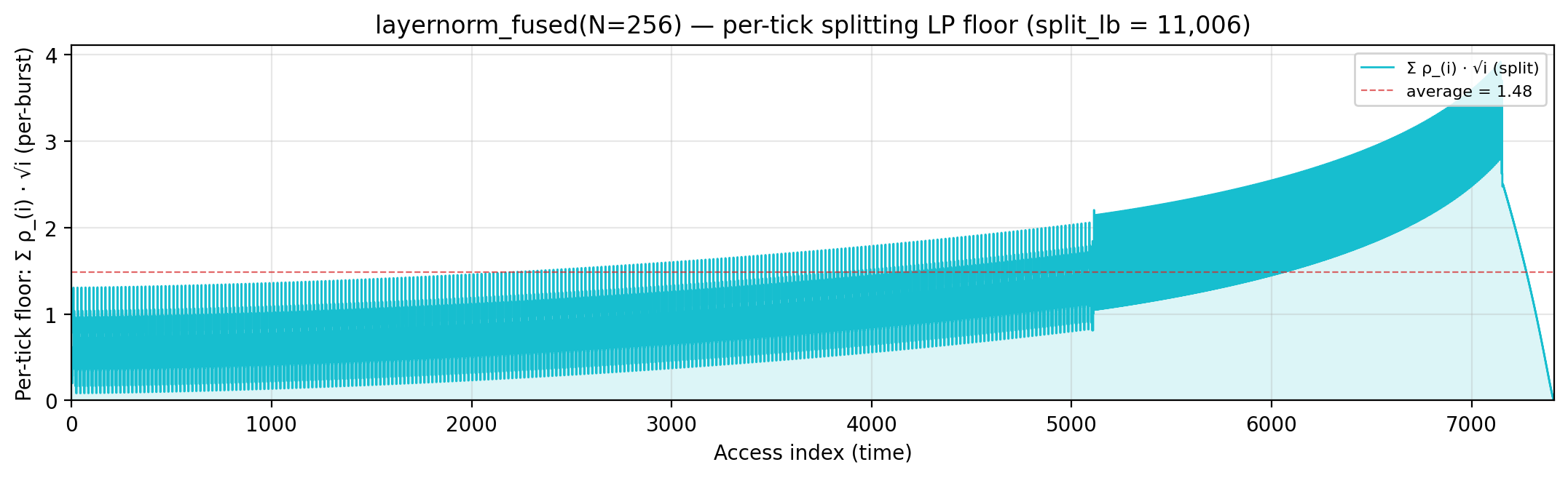
Per-tick polymatroid LP floor — integrand of polymatroid_lb: Σ_v reads_v · ⌈√d_v⌉ / lifespan(v) over live vars, where d_v is each variable’s LP-implied static depth (gemini/polymatroid-relaxation.md). The area equals the geometric portion of polymatroid_lb.
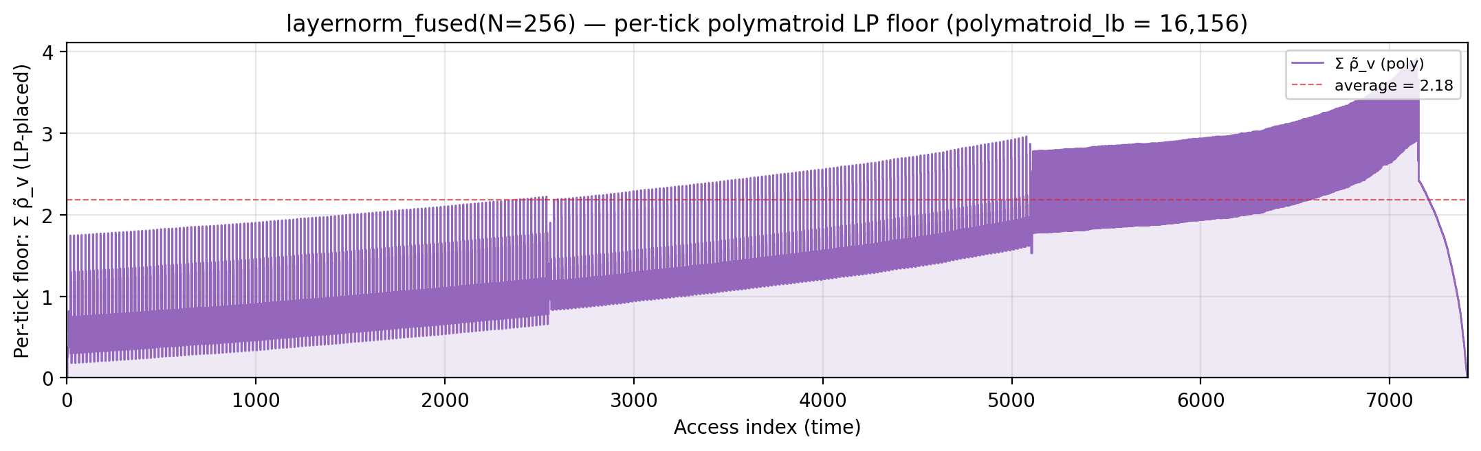
Rolling spatial intensity — heartbeat plot of ops / Σ ⌈√d⌉ over a sliding window.
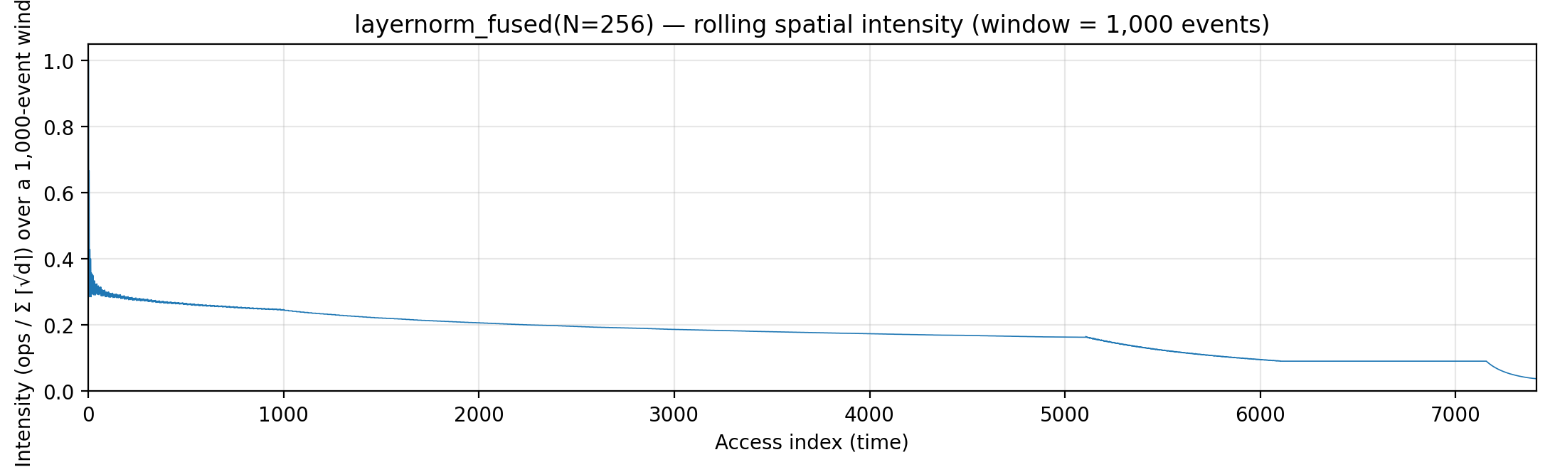
Cumulative compute vs fetch cost — slope = instantaneous spatial arithmetic intensity.
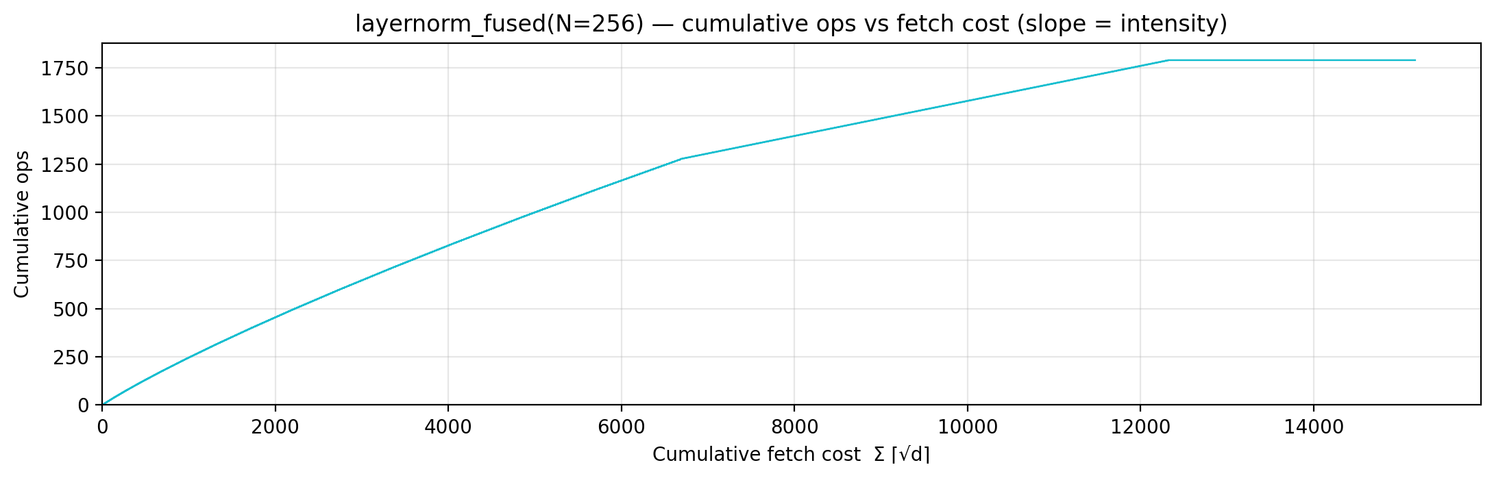
Gravity well — per-load fetch-cost ⌈√d⌉ scatter.
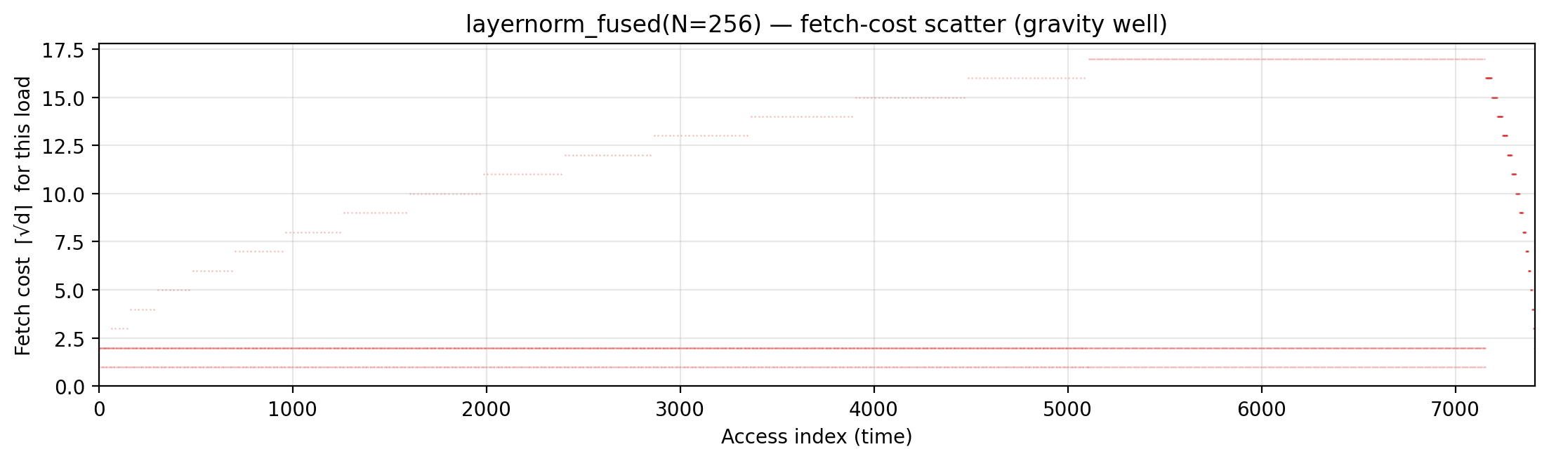
Spatial locality CDF — compute-fulfillment as a function of radius.
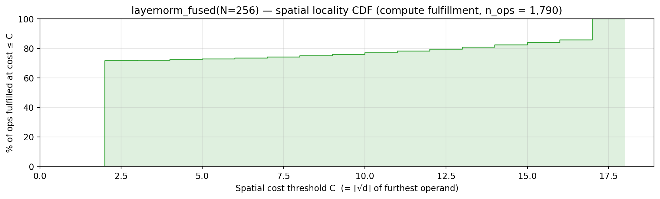
Working-set size over a τ = 193-event window (max = 193).
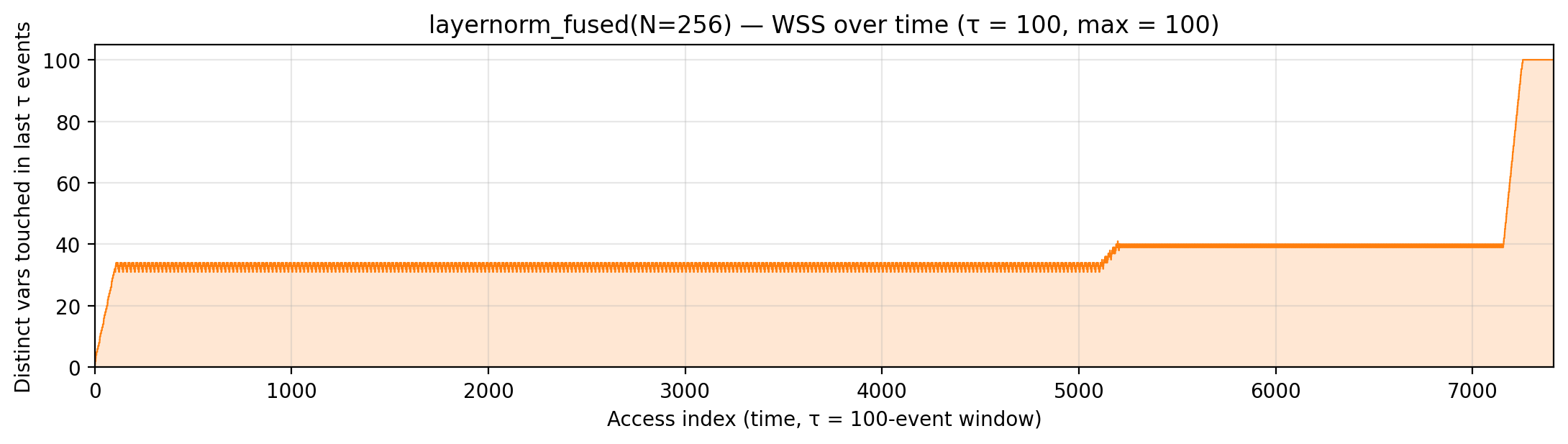
matrix_powers_naive (code)
n=16, s=4. Algorithm. Run matvec s times — x₁=Ax₀, x₂=Ax₁, …. A is re-read in full every step.
Manual. A on arg stack so re-reads are priced identically each time; the naive cost is dominated by the fixed arg-stack positions of A.
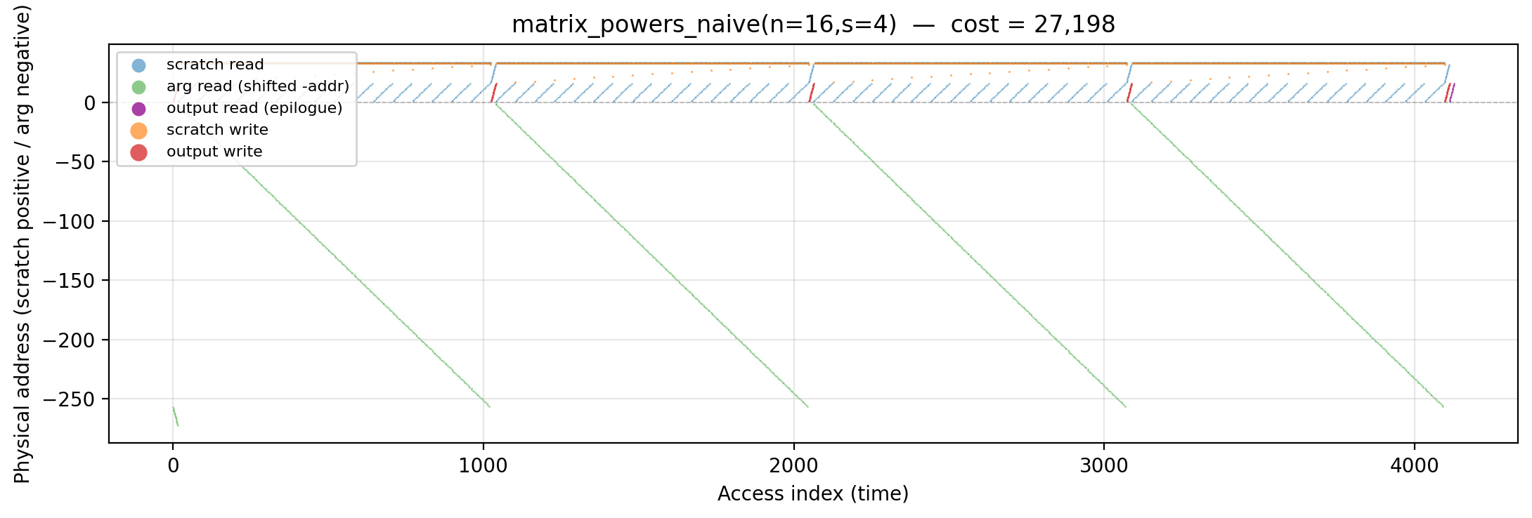
Working-set size over time (peak = 288).
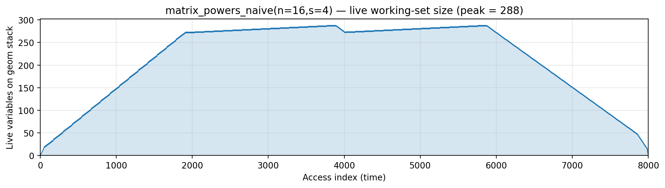
Reuse distance per load — LRU vs Bélády OPT (max LRU = 287; max OPT = 272).
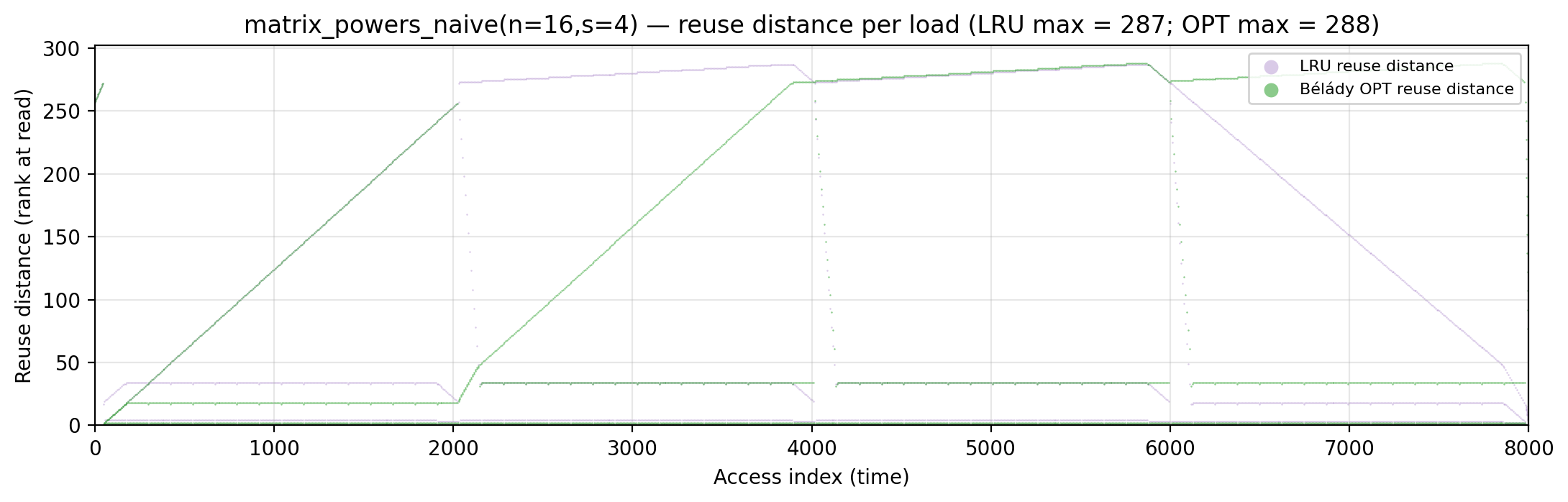
Miss-ratio curve — LRU vs Bélády OPT misses by cache capacity.
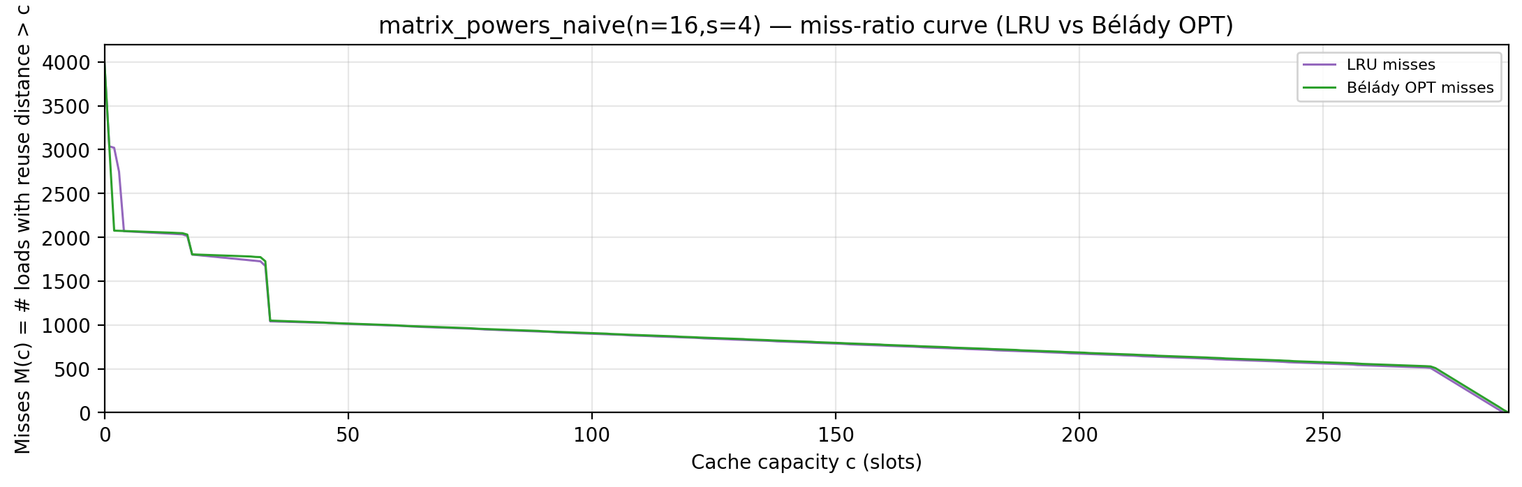
Per-tick TU LP floor — integrand of global_density: Σ_i ρ_{(i)} · √i over currently-live vars, ranked by density; the area equals global_density.
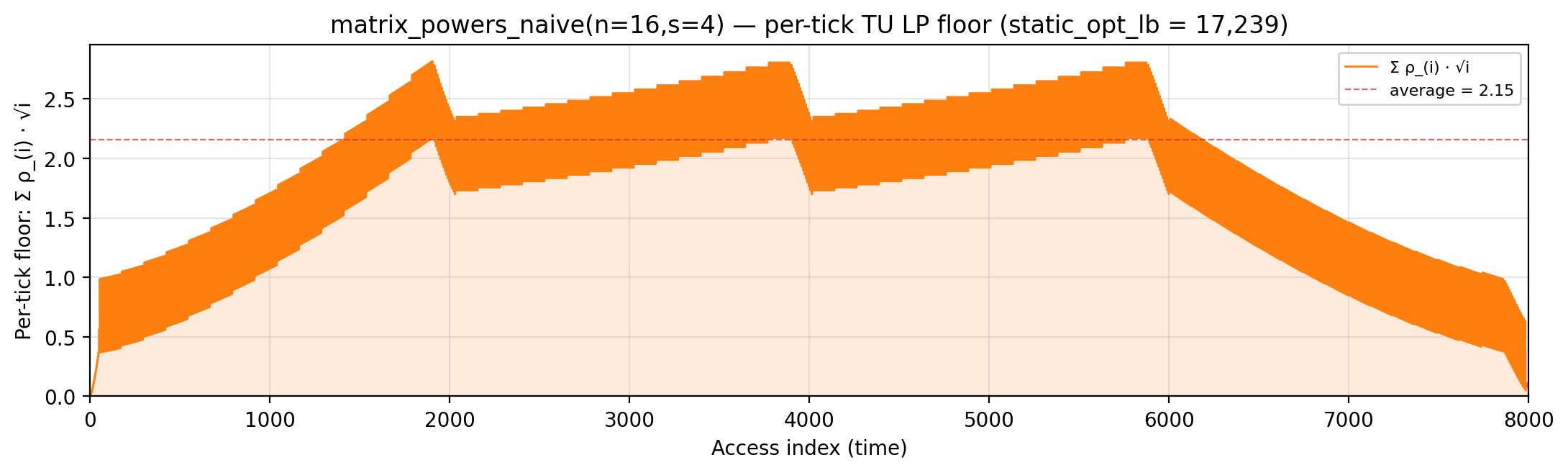
Per-tick splitting LP floor — integrand of local_density: Σ_i ρ_{(i)} · √i over the currently-active per-burst virtual intervals; the area equals the geometric portion of local_density.
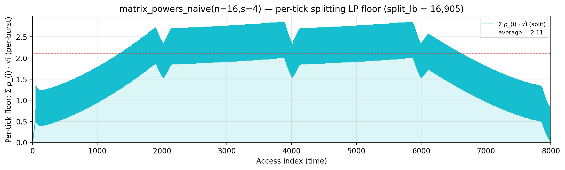
Per-tick polymatroid LP floor — integrand of polymatroid_lb: Σ_v reads_v · ⌈√d_v⌉ / lifespan(v) over live vars, where d_v is each variable’s LP-implied static depth (gemini/polymatroid-relaxation.md). The area equals the geometric portion of polymatroid_lb.
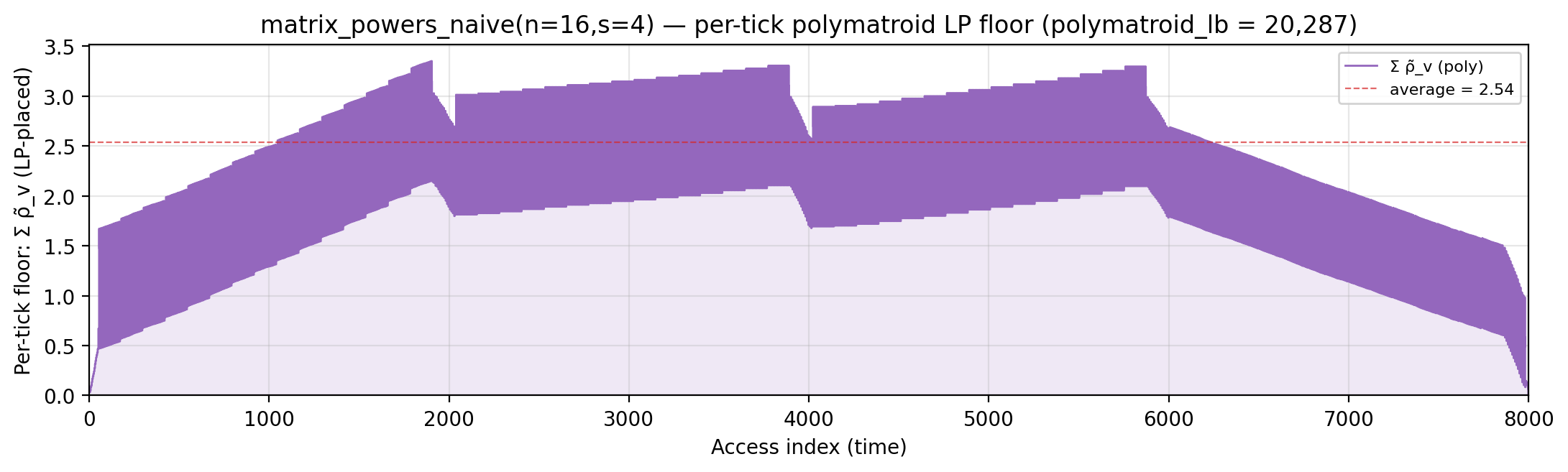
Rolling spatial intensity — heartbeat plot of ops / Σ ⌈√d⌉ over a sliding window.
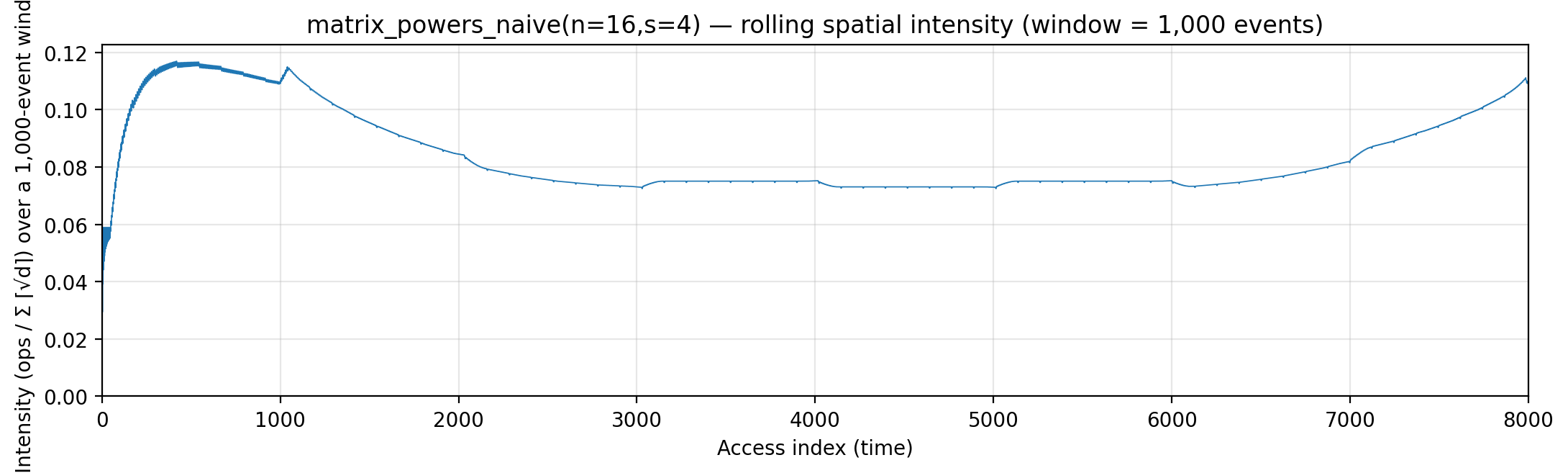
Cumulative compute vs fetch cost — slope = instantaneous spatial arithmetic intensity.
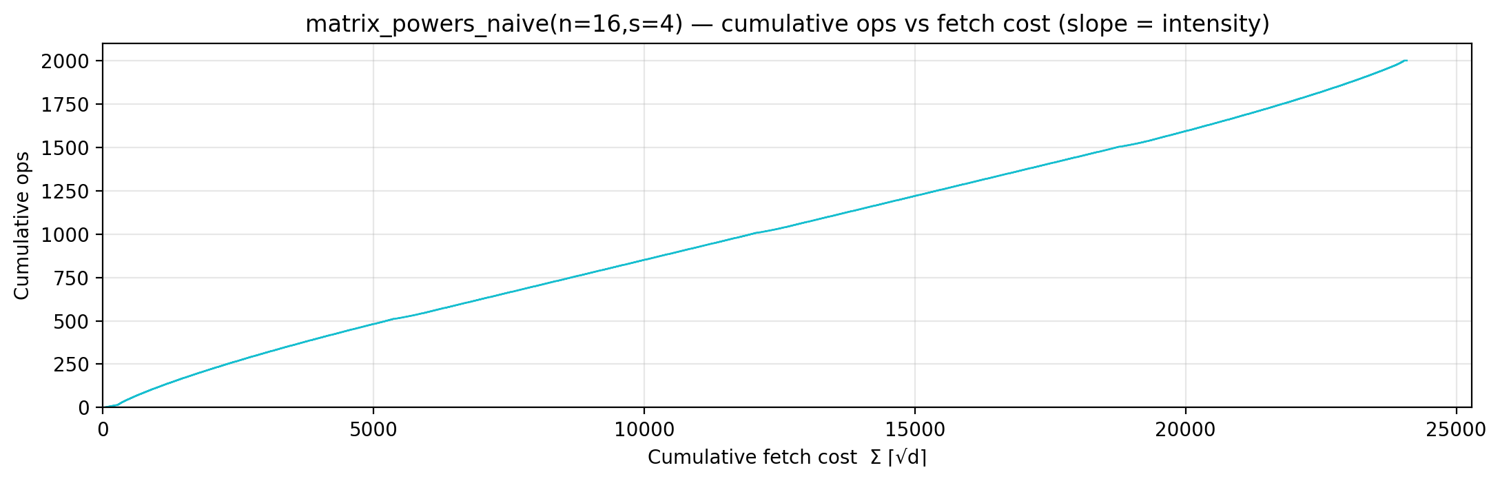
Gravity well — per-load fetch-cost ⌈√d⌉ scatter.
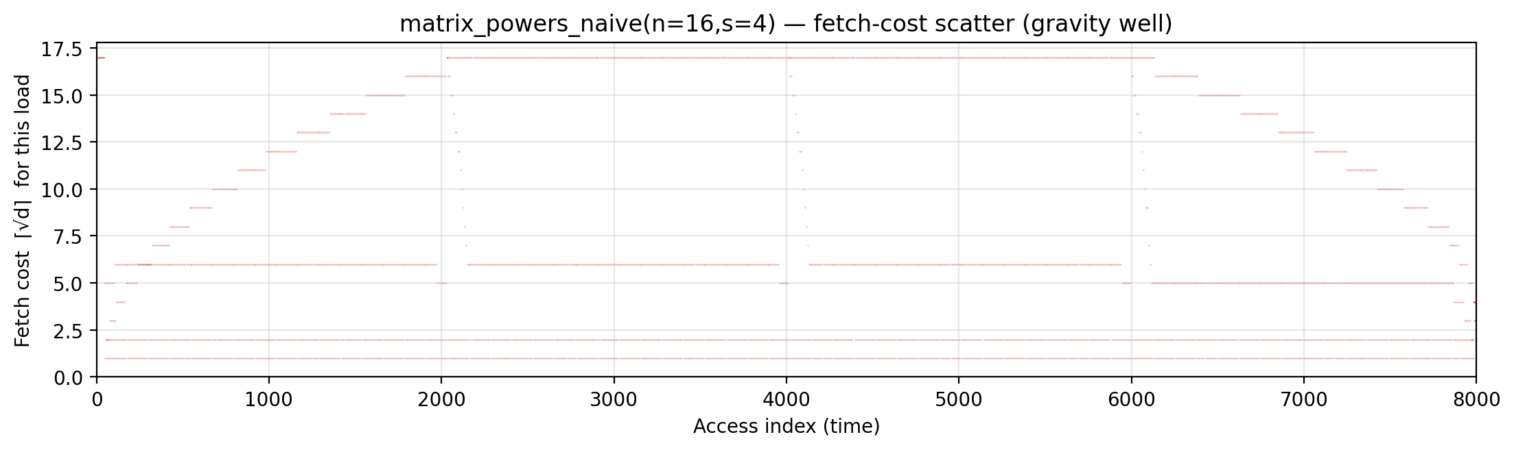
Spatial locality CDF — compute-fulfillment as a function of radius.
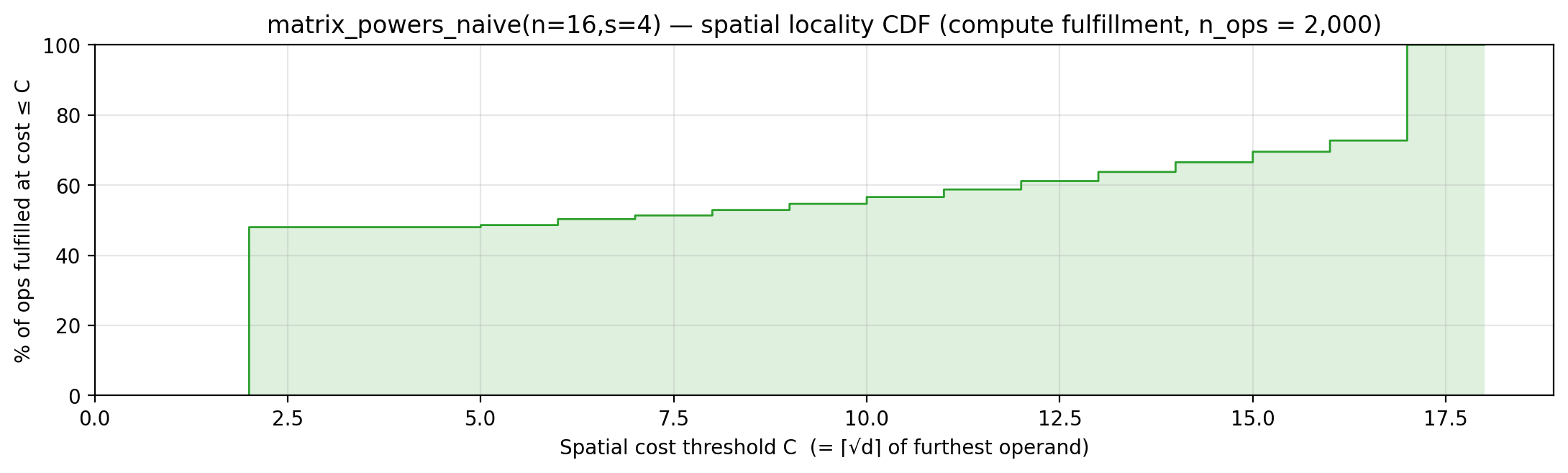
Working-set size over a τ = 276-event window (max = 137).
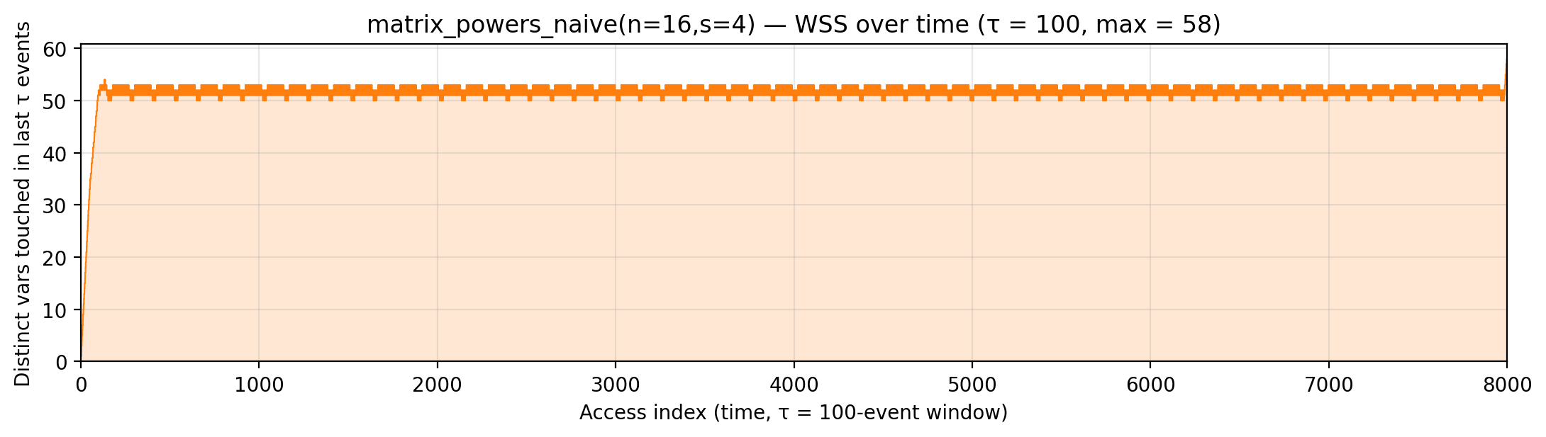
matrix_powers_ca (code)
n=16, s=4, block=4. Algorithm. Communication-avoiding s-step: process A in row-blocks; for each block compute all step outputs locally before moving on.
Manual. Under the two-stack model A already lives on the arg stack with fixed per-position cost, so the CA benefit cannot amortize. Cost matches naive — heuristic differences come from the re-order of the events.
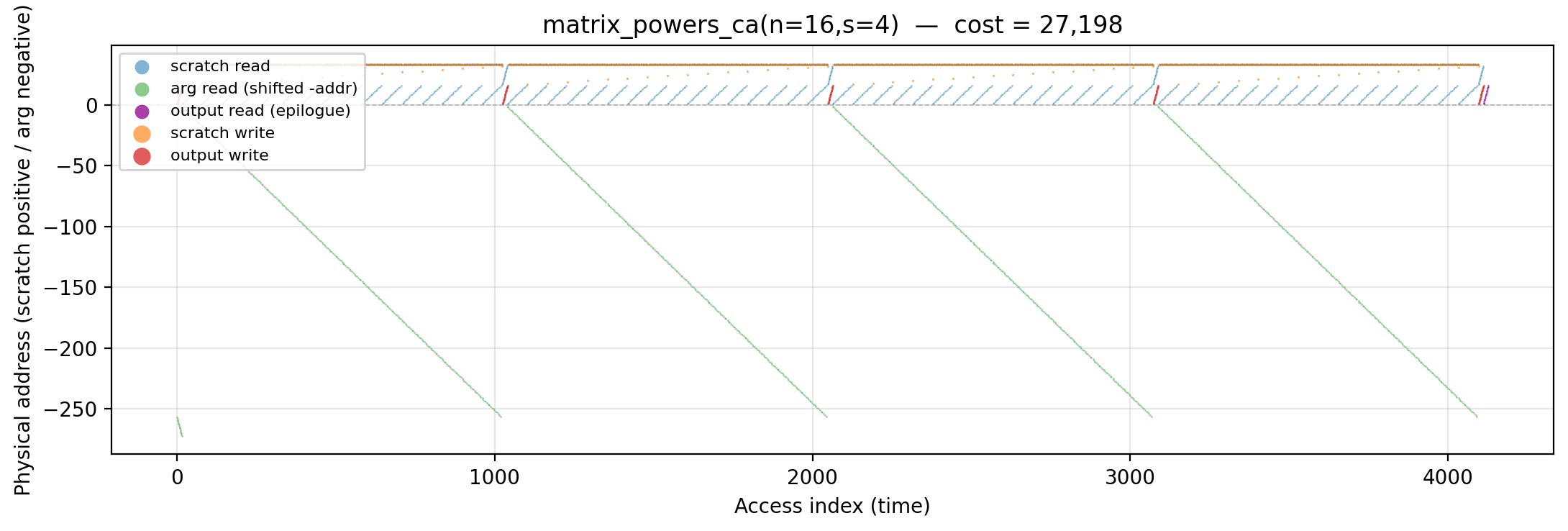
Working-set size over time (peak = 288).
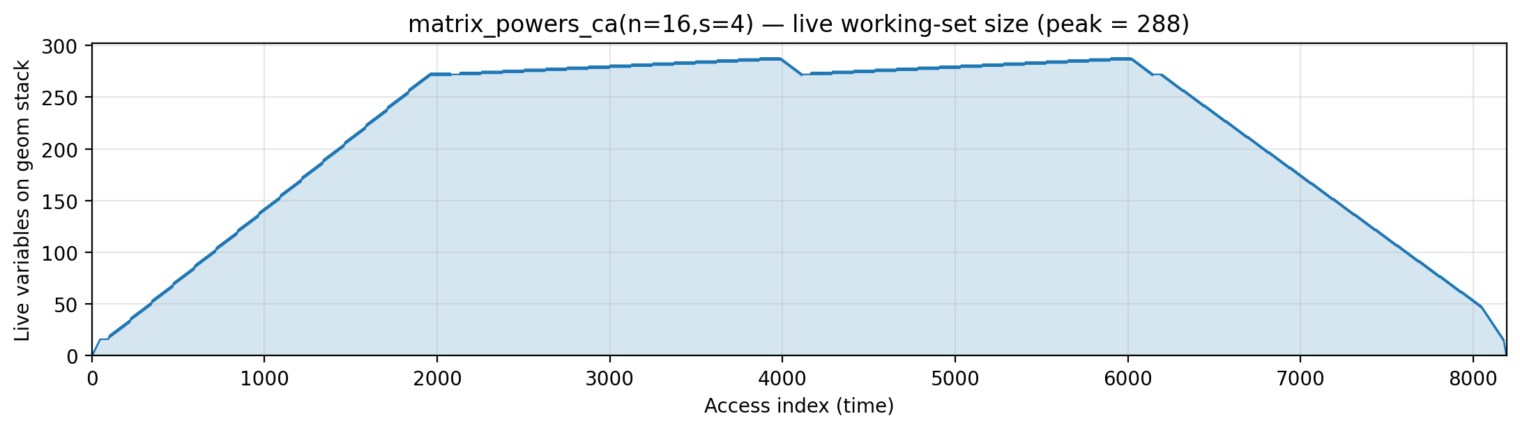
Reuse distance per load — LRU vs Bélády OPT (max LRU = 287; max OPT = 272).
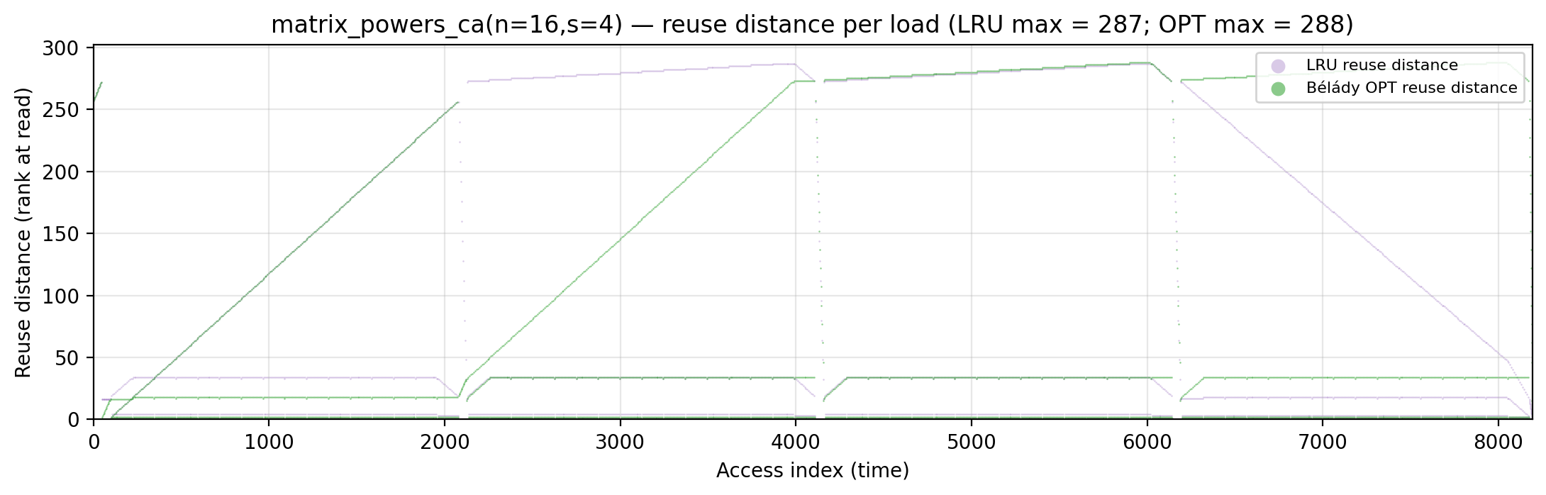
Miss-ratio curve — LRU vs Bélády OPT misses by cache capacity.
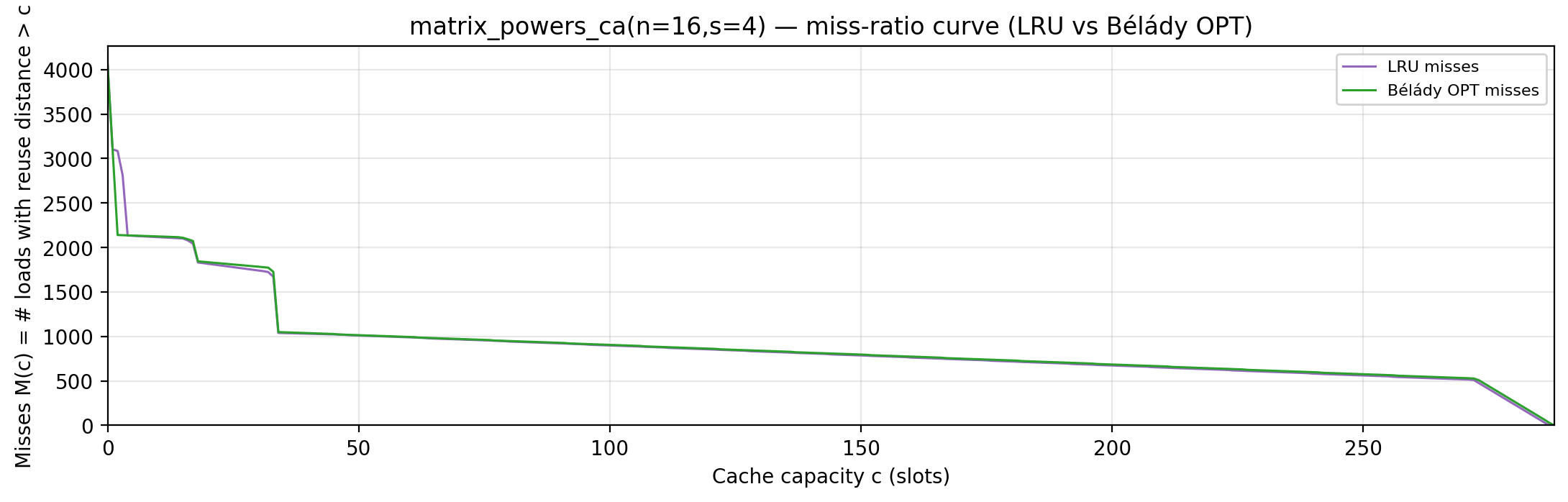
Per-tick TU LP floor — integrand of global_density: Σ_i ρ_{(i)} · √i over currently-live vars, ranked by density; the area equals global_density.
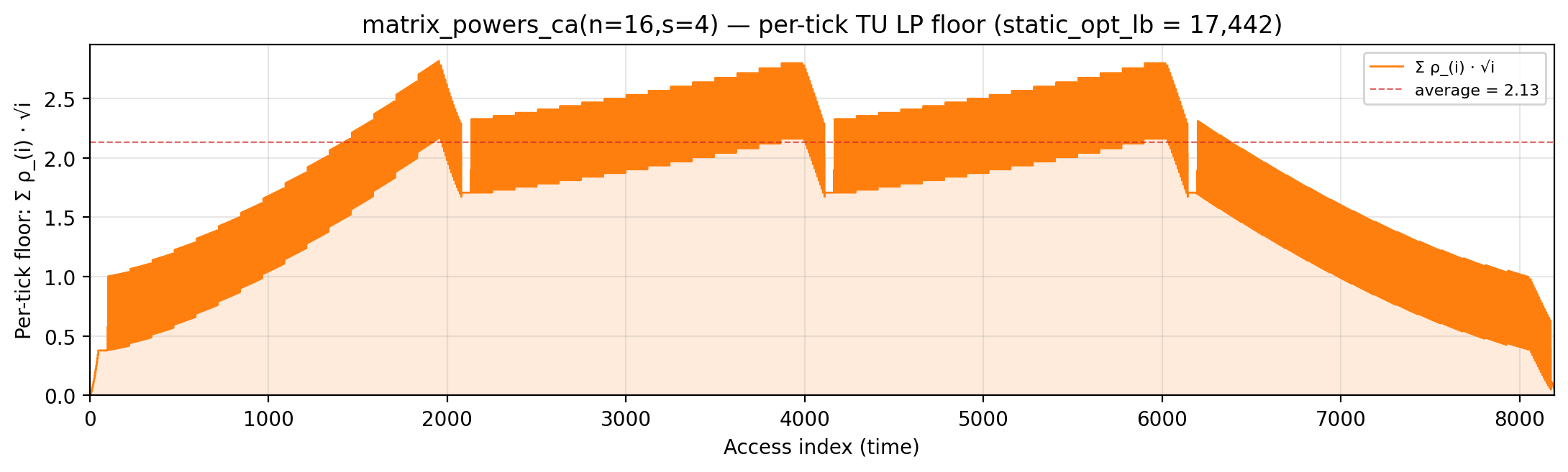
Per-tick splitting LP floor — integrand of local_density: Σ_i ρ_{(i)} · √i over the currently-active per-burst virtual intervals; the area equals the geometric portion of local_density.
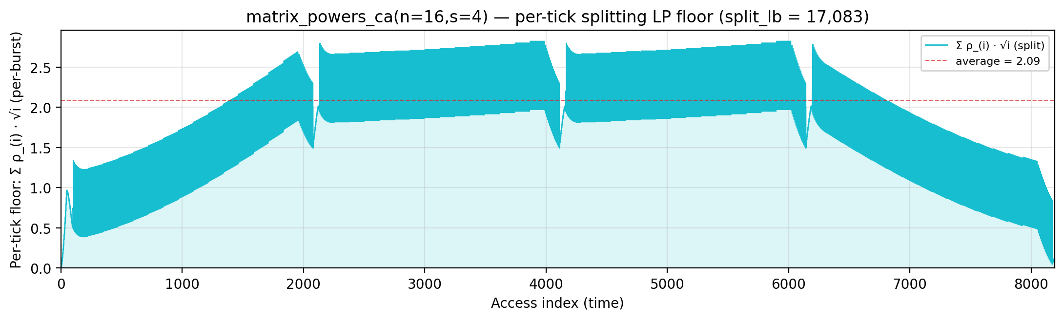
Per-tick polymatroid LP floor — integrand of polymatroid_lb: Σ_v reads_v · ⌈√d_v⌉ / lifespan(v) over live vars, where d_v is each variable’s LP-implied static depth (gemini/polymatroid-relaxation.md). The area equals the geometric portion of polymatroid_lb.
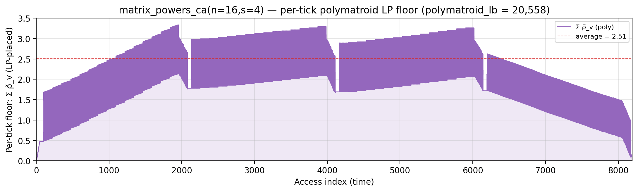
Rolling spatial intensity — heartbeat plot of ops / Σ ⌈√d⌉ over a sliding window.
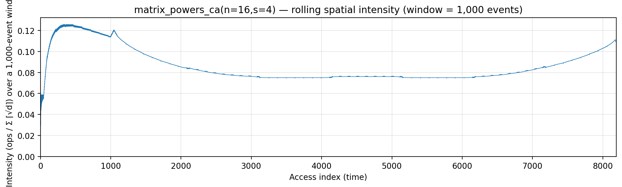
Cumulative compute vs fetch cost — slope = instantaneous spatial arithmetic intensity.
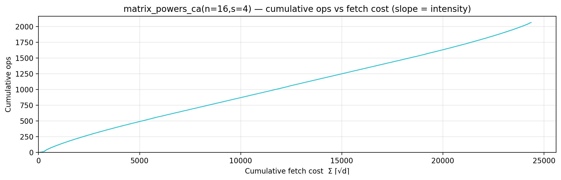
Gravity well — per-load fetch-cost ⌈√d⌉ scatter.
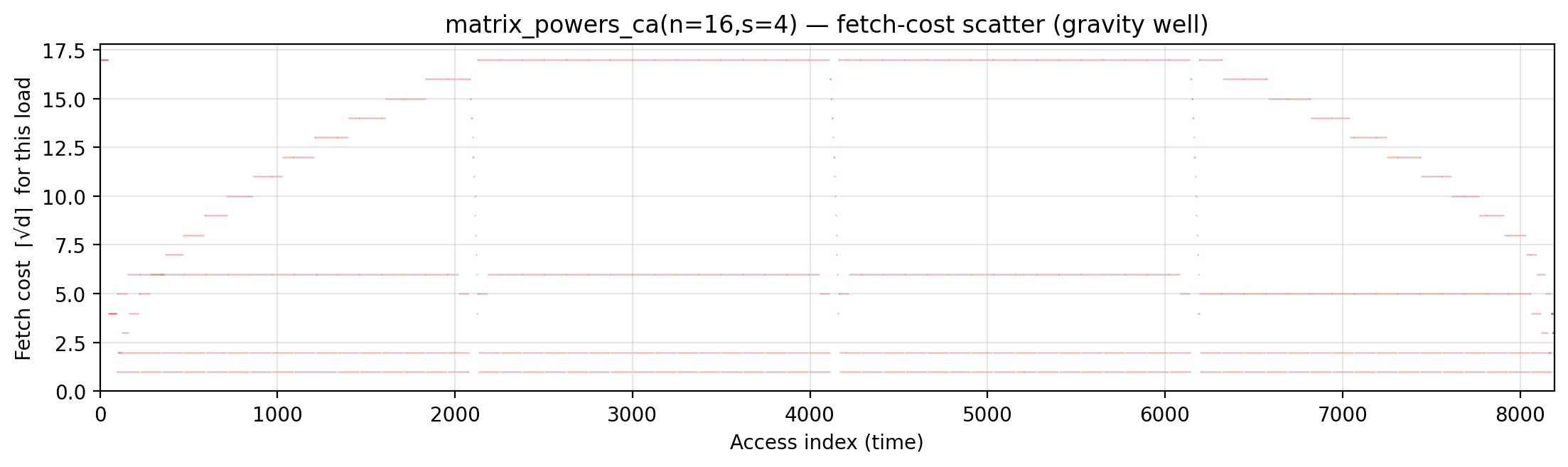
Spatial locality CDF — compute-fulfillment as a function of radius.
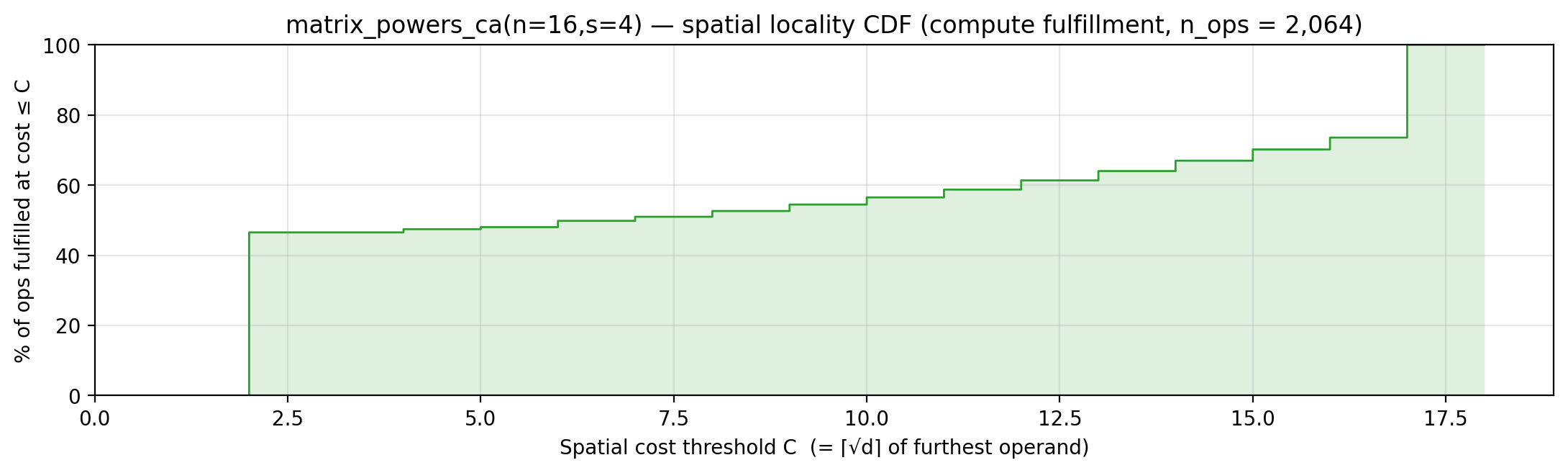
Working-set size over a τ = 276-event window (max = 134).
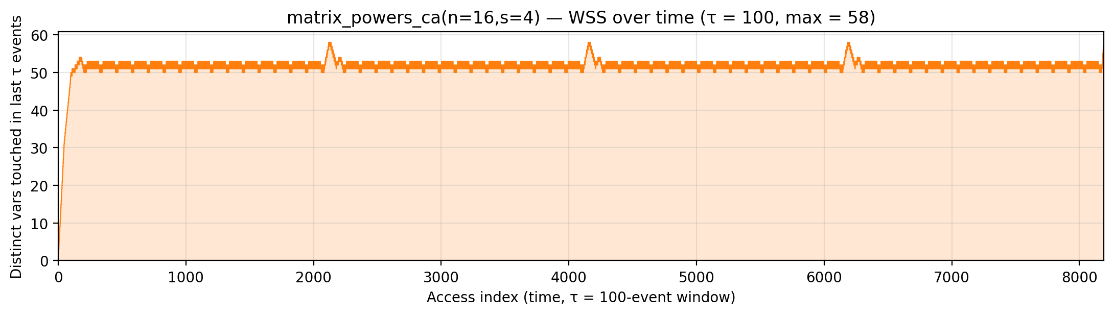
cholesky_left_looking (code)
n=32. Algorithm. Complement of the default right-looking Cholesky: for column k pull data from all previously-factored columns 0..k-1 (far-flung reads), then finalize column k locally (concentrated writes).
Manual. Two hoisted scratchpads with lazy arg-stack reads: c_A
(addr 1) pins the accumulator L[i][k] during the past-factor
sweep; c_C (addrs 2..n+1) caches row k’s previously-factored tail
L[k][0..k-1]. Inner L[i][k] += L[i][j] * L[k][j] body reads one
bulk cell (the past factor L[i][j]) and two hot scratchpads.
Drops manual from 494,000 to 244,300 (−51%), still above
global_density (112,864) but well below bytedmd_classic (352,335).
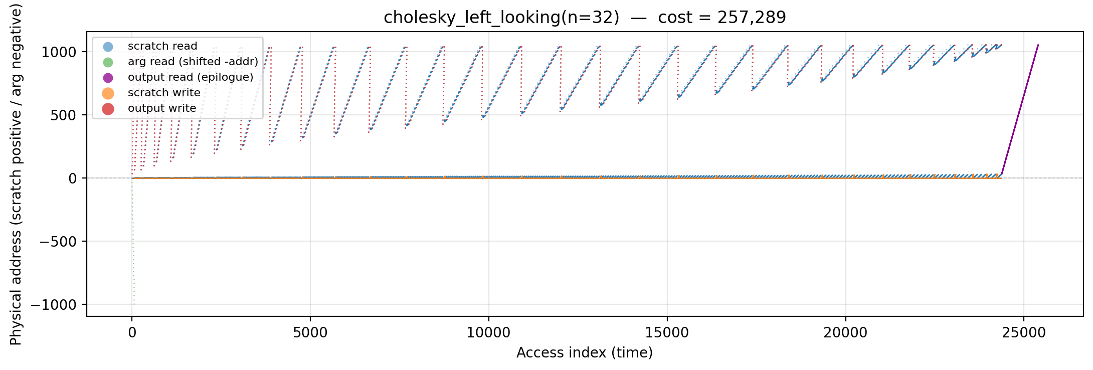
Working-set size over time (peak = 1,025).
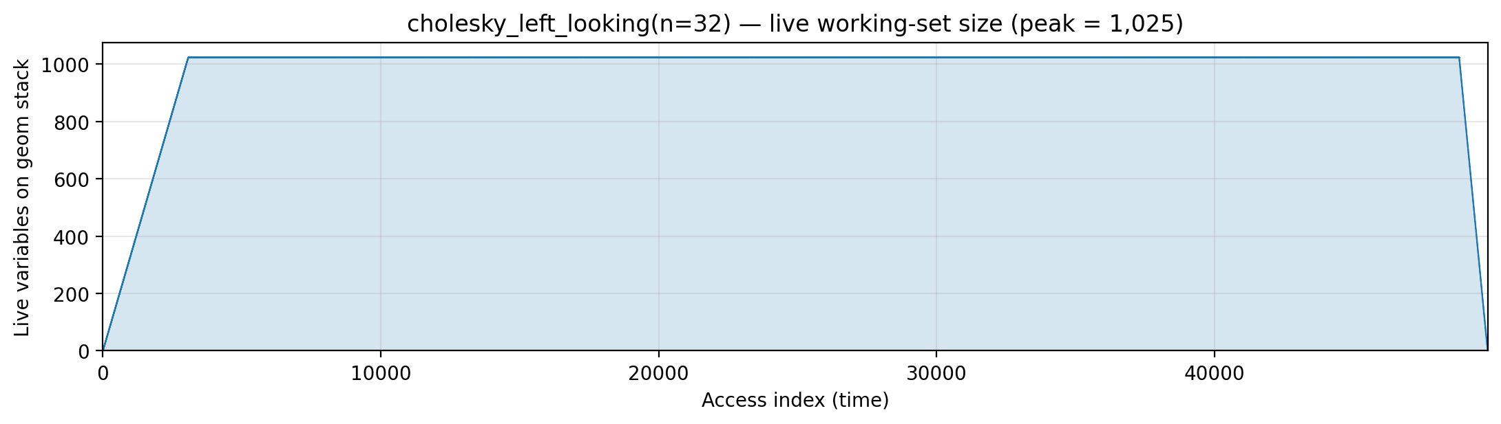
Reuse distance per load — LRU vs Bélády OPT (max LRU = 1,024; max OPT = 1,024).
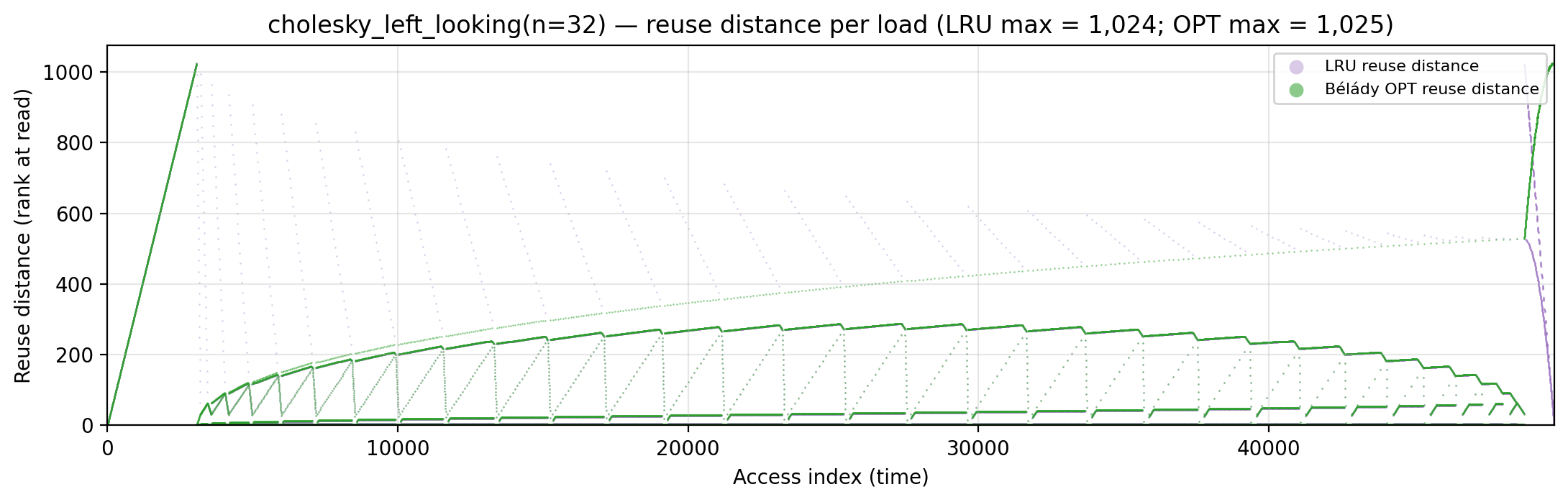
Miss-ratio curve — LRU vs Bélády OPT misses by cache capacity.
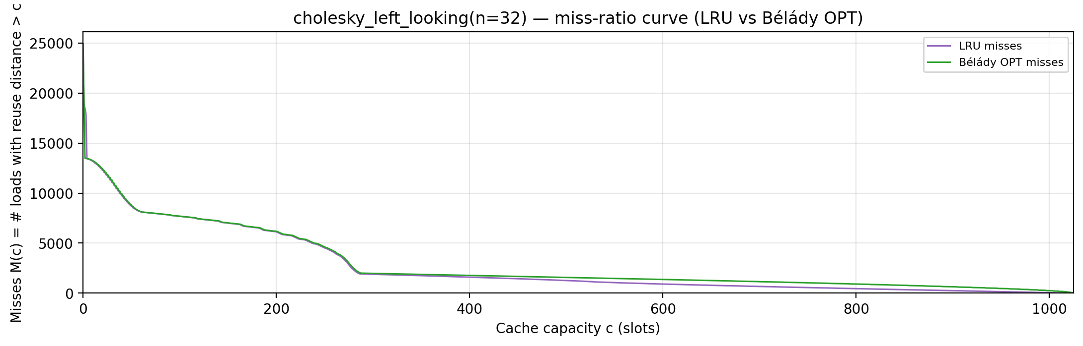
Per-tick TU LP floor — integrand of global_density: Σ_i ρ_{(i)} · √i over currently-live vars, ranked by density; the area equals global_density.
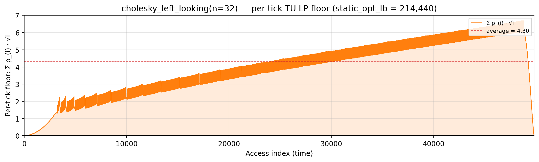
Per-tick splitting LP floor — integrand of local_density: Σ_i ρ_{(i)} · √i over the currently-active per-burst virtual intervals; the area equals the geometric portion of local_density.
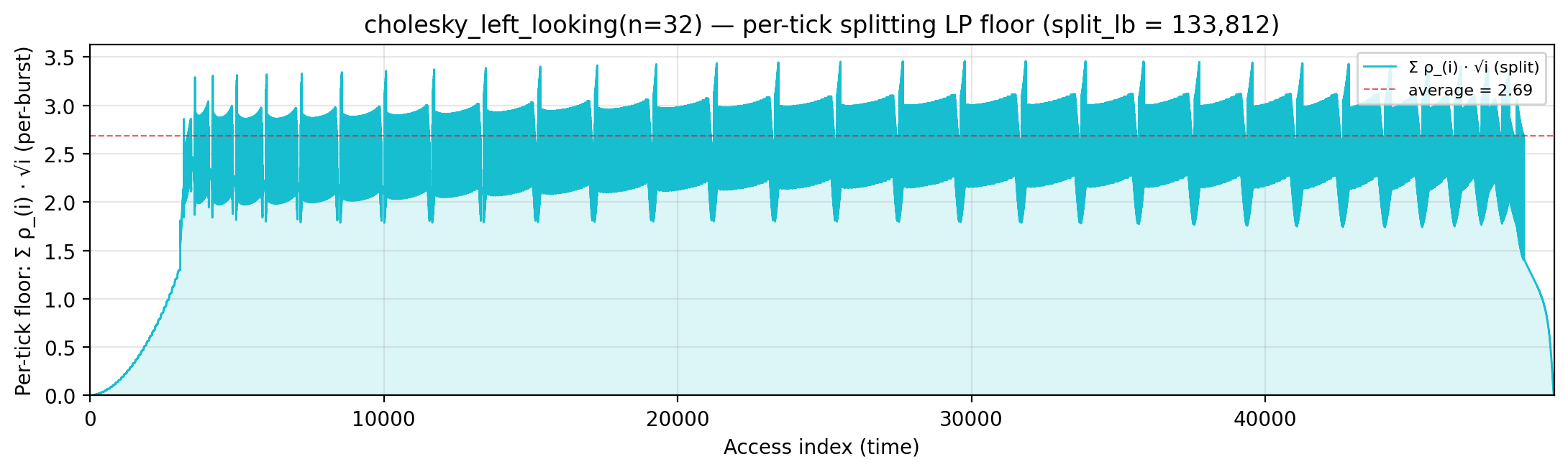
Rolling spatial intensity — heartbeat plot of ops / Σ ⌈√d⌉ over a sliding window.
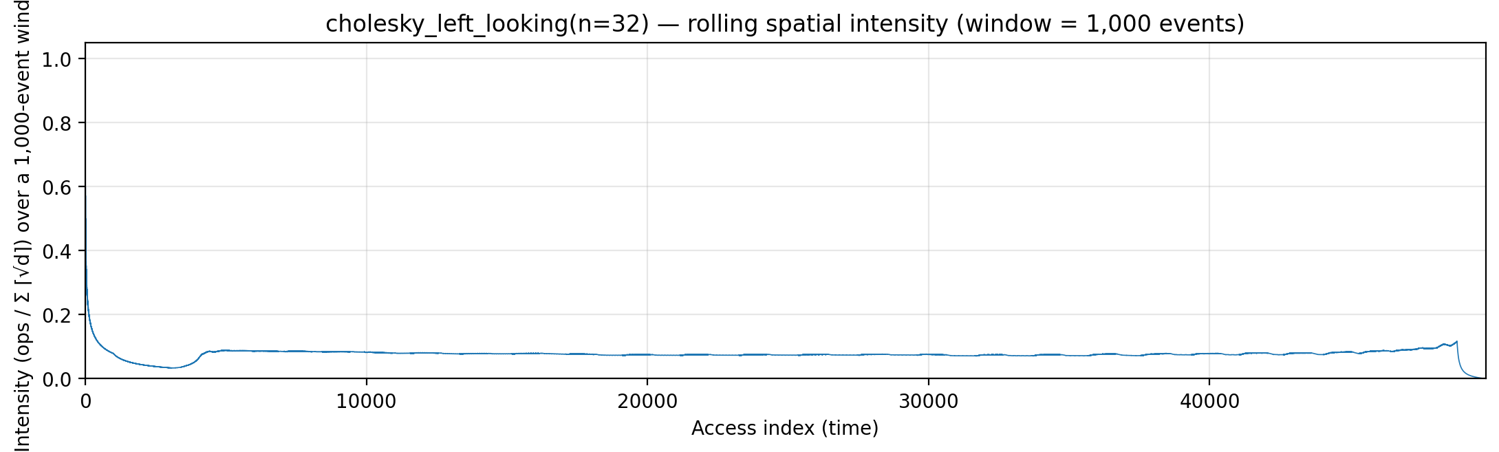
Cumulative compute vs fetch cost — slope = instantaneous spatial arithmetic intensity.
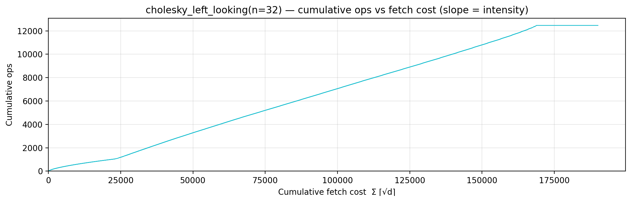
Gravity well — per-load fetch-cost ⌈√d⌉ scatter.
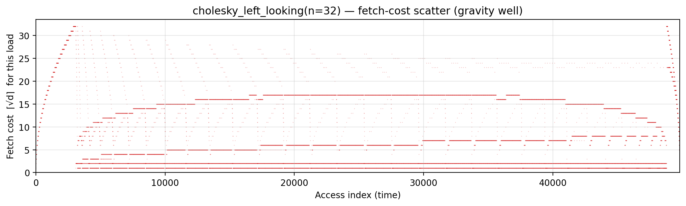
Spatial locality CDF — compute-fulfillment as a function of radius.
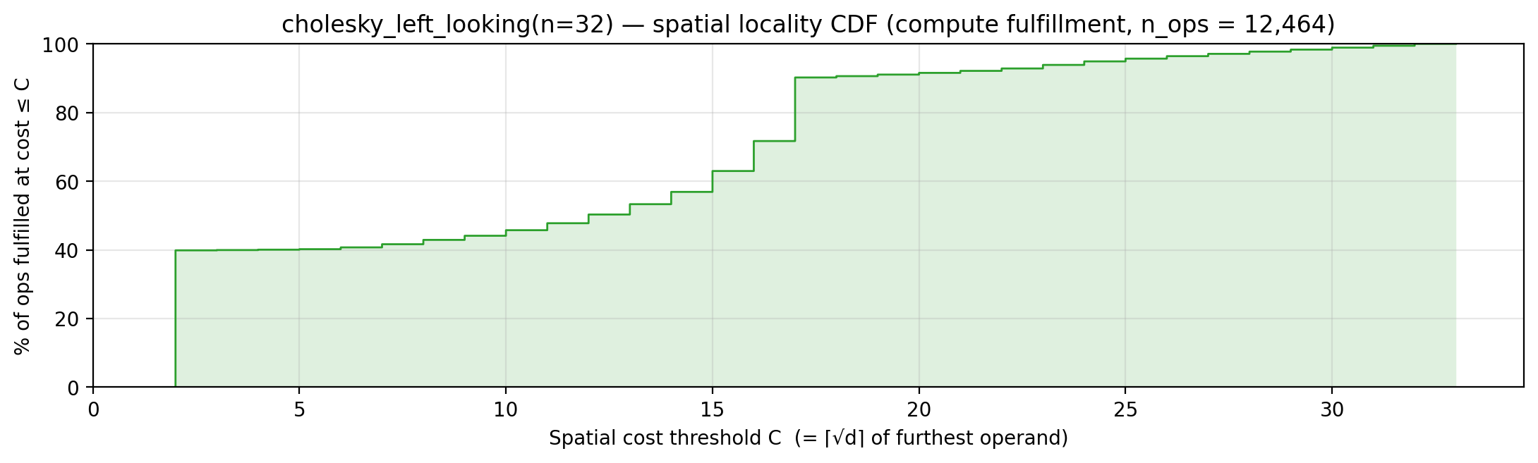
Working-set size over a τ = 279-event window (max = 279).
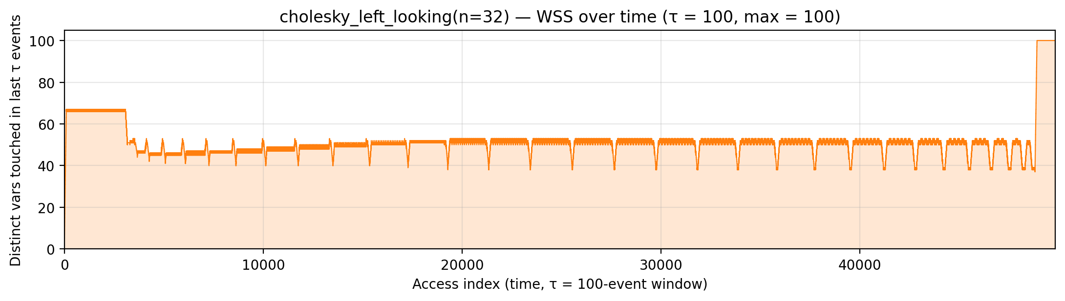
spmv_csr_banded (code)
n=32, bandwidth=3. Algorithm. Sparse matvec with CSR indices clustered near the diagonal. col_ind is a compile-time array (no memory cost), x-reads are data-dependent but spatially local.
Manual. vals and x on arg stack; accumulator and y on scratch.
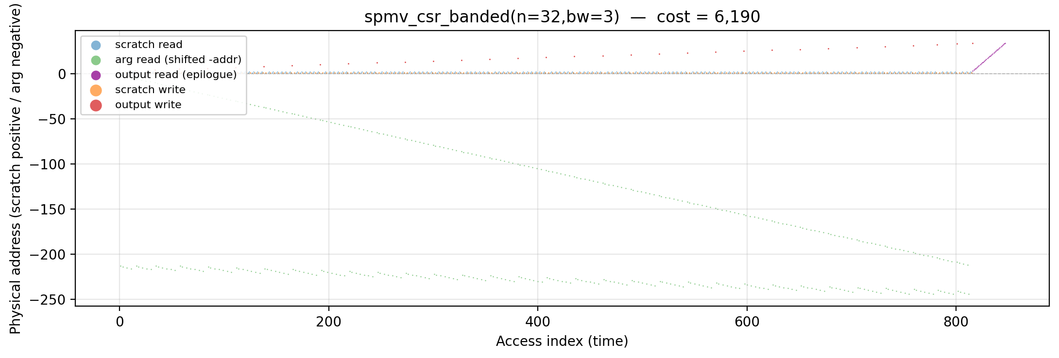
Working-set size over time (peak = 214).
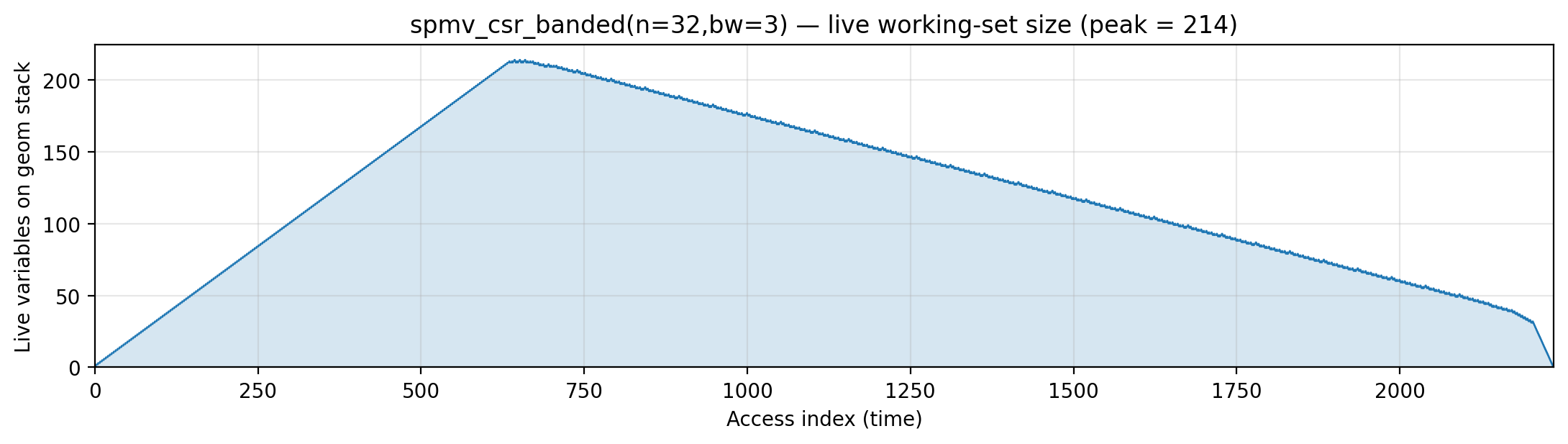
Reuse distance per load — LRU vs Bélády OPT (max LRU = 213; max OPT = 32).
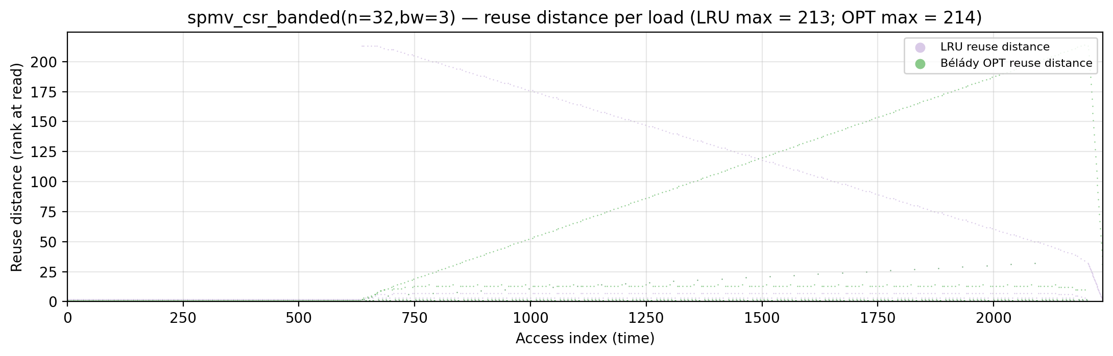
Miss-ratio curve — LRU vs Bélády OPT misses by cache capacity.
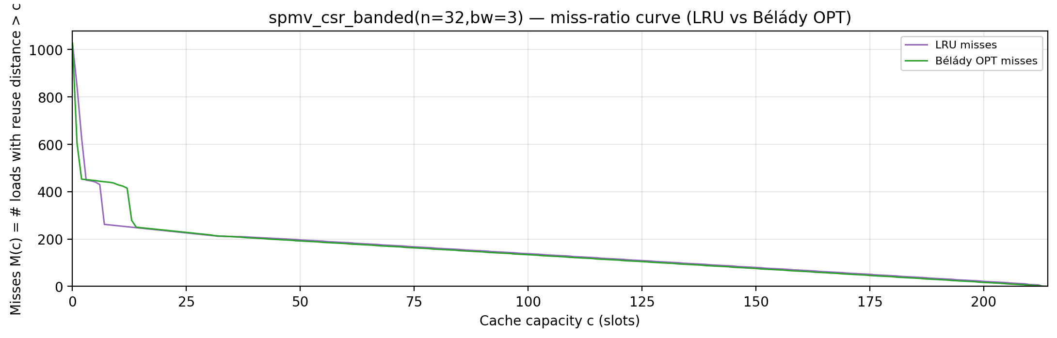
Per-tick TU LP floor — integrand of global_density: Σ_i ρ_{(i)} · √i over currently-live vars, ranked by density; the area equals global_density.
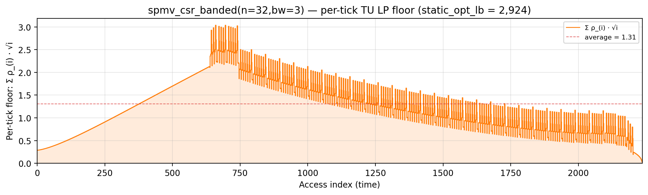
Per-tick splitting LP floor — integrand of local_density: Σ_i ρ_{(i)} · √i over the currently-active per-burst virtual intervals; the area equals the geometric portion of local_density.
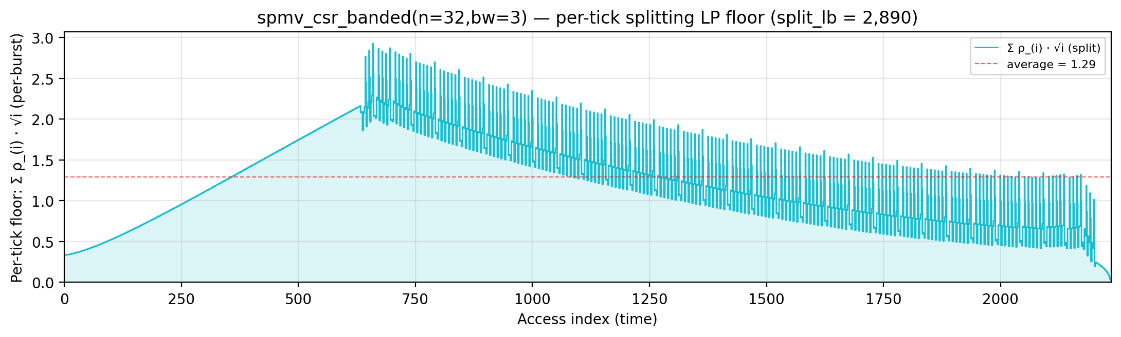
Per-tick polymatroid LP floor — integrand of polymatroid_lb: Σ_v reads_v · ⌈√d_v⌉ / lifespan(v) over live vars, where d_v is each variable’s LP-implied static depth (gemini/polymatroid-relaxation.md). The area equals the geometric portion of polymatroid_lb.

Rolling spatial intensity — heartbeat plot of ops / Σ ⌈√d⌉ over a sliding window.
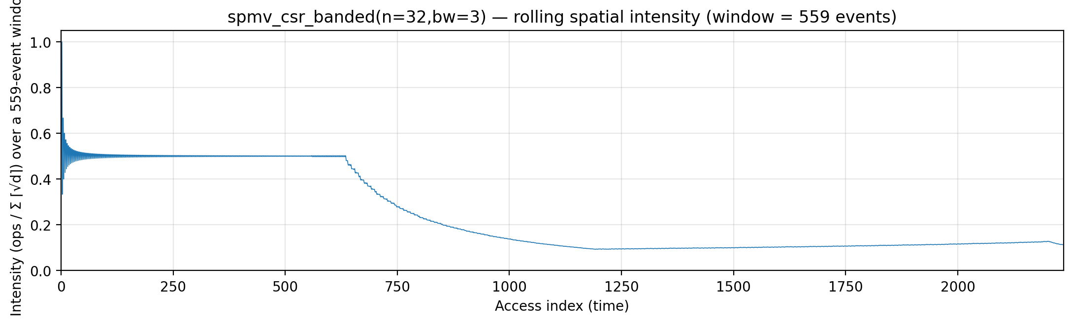
Cumulative compute vs fetch cost — slope = instantaneous spatial arithmetic intensity.
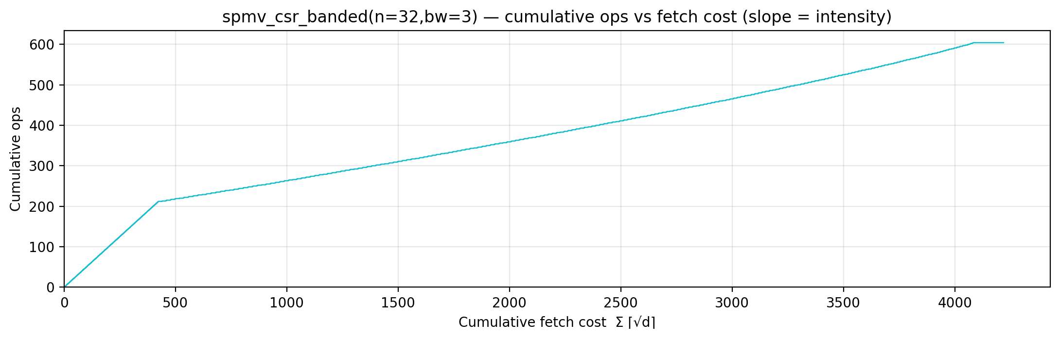
Gravity well — per-load fetch-cost ⌈√d⌉ scatter.

Spatial locality CDF — compute-fulfillment as a function of radius.
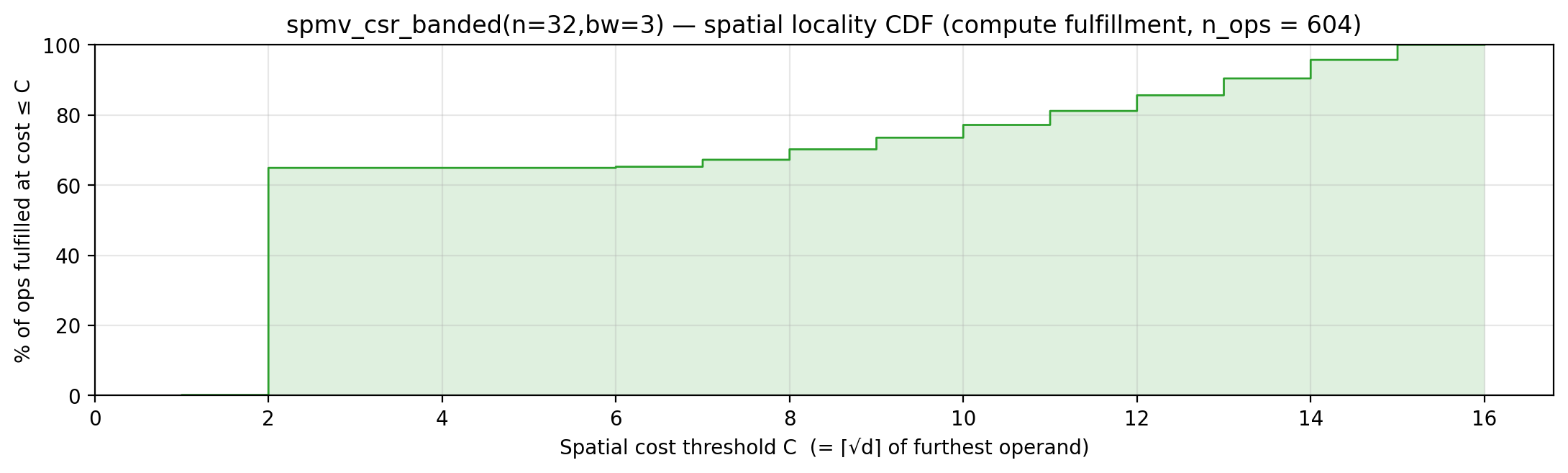
Working-set size over a τ = 131-event window (max = 74).
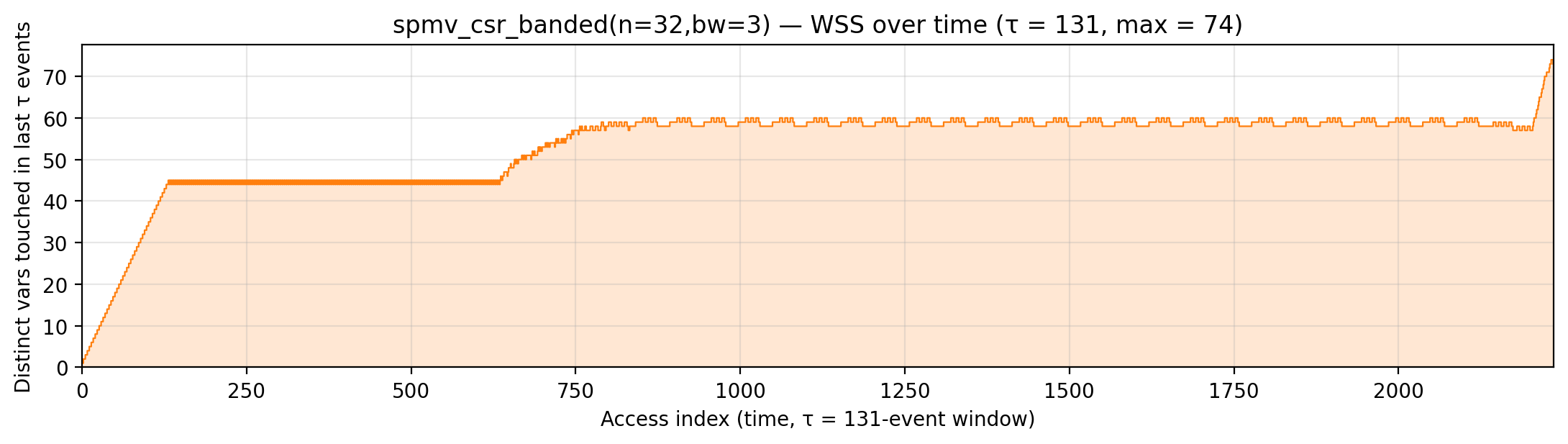
spmv_csr_random (code)
n=32, nnz/row=7. Algorithm. Same CSR machinery as banded but col_ind is a random Erdős-Rényi pattern. x-reads scatter all over the vector, which LRU heuristics penalize while density ranking can still pin hot nodes.
Manual. Identical layout to banded; the cost difference comes from which arg-stack positions of x get read how often.
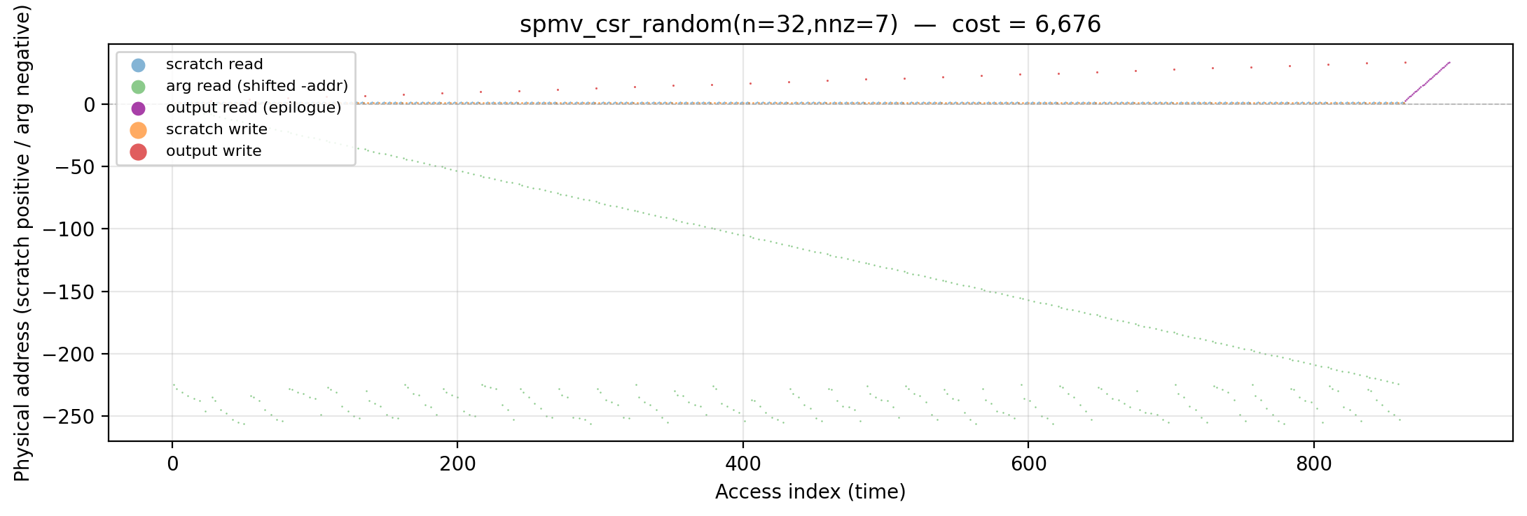
Working-set size over time (peak = 226).
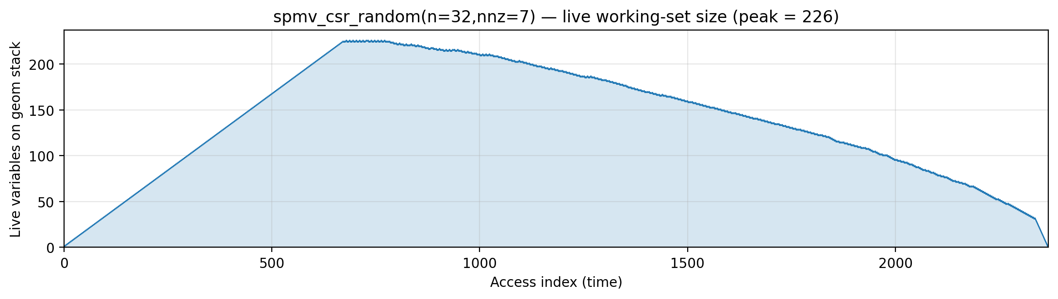
Reuse distance per load — LRU vs Bélády OPT (max LRU = 226; max OPT = 32).

Miss-ratio curve — LRU vs Bélády OPT misses by cache capacity.
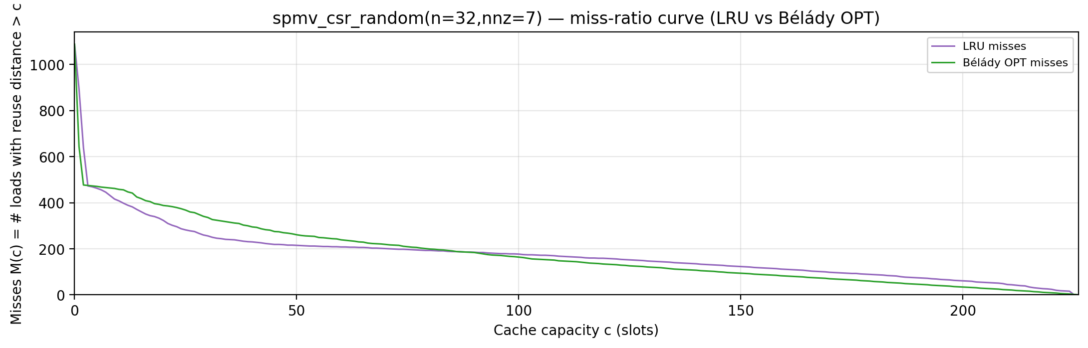
Per-tick TU LP floor — integrand of global_density: Σ_i ρ_{(i)} · √i over currently-live vars, ranked by density; the area equals global_density.
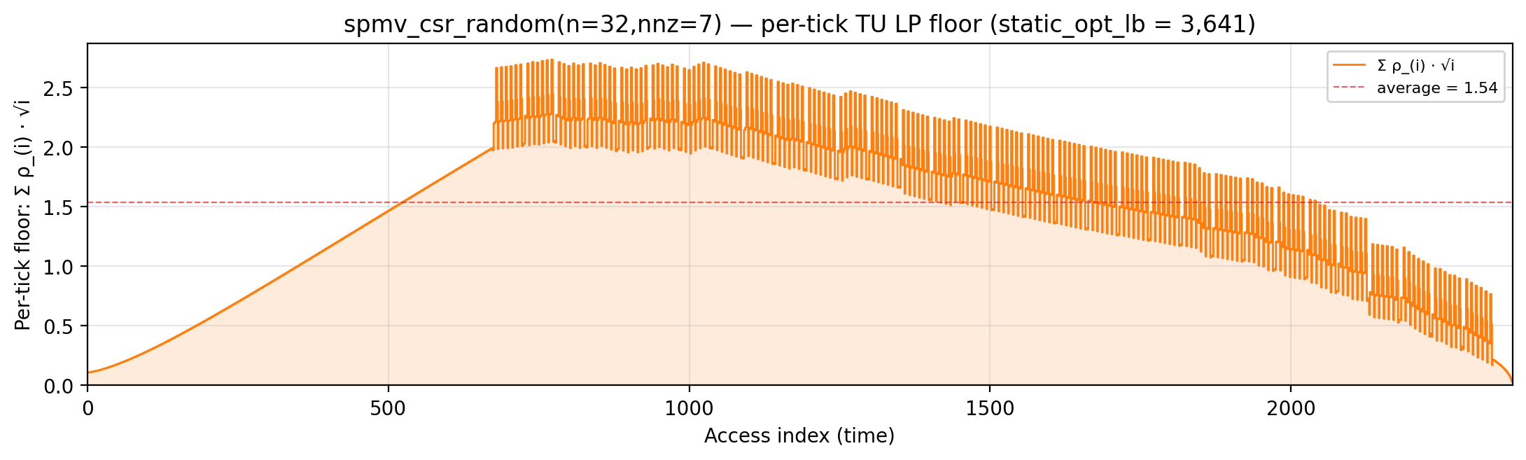
Per-tick splitting LP floor — integrand of local_density: Σ_i ρ_{(i)} · √i over the currently-active per-burst virtual intervals; the area equals the geometric portion of local_density.
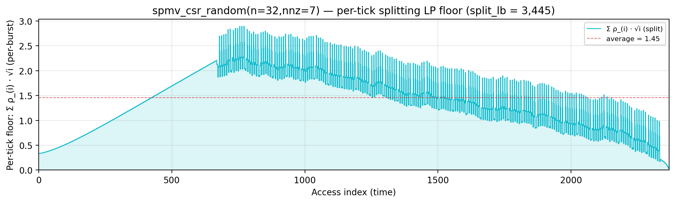
Per-tick polymatroid LP floor — integrand of polymatroid_lb: Σ_v reads_v · ⌈√d_v⌉ / lifespan(v) over live vars, where d_v is each variable’s LP-implied static depth (gemini/polymatroid-relaxation.md). The area equals the geometric portion of polymatroid_lb.
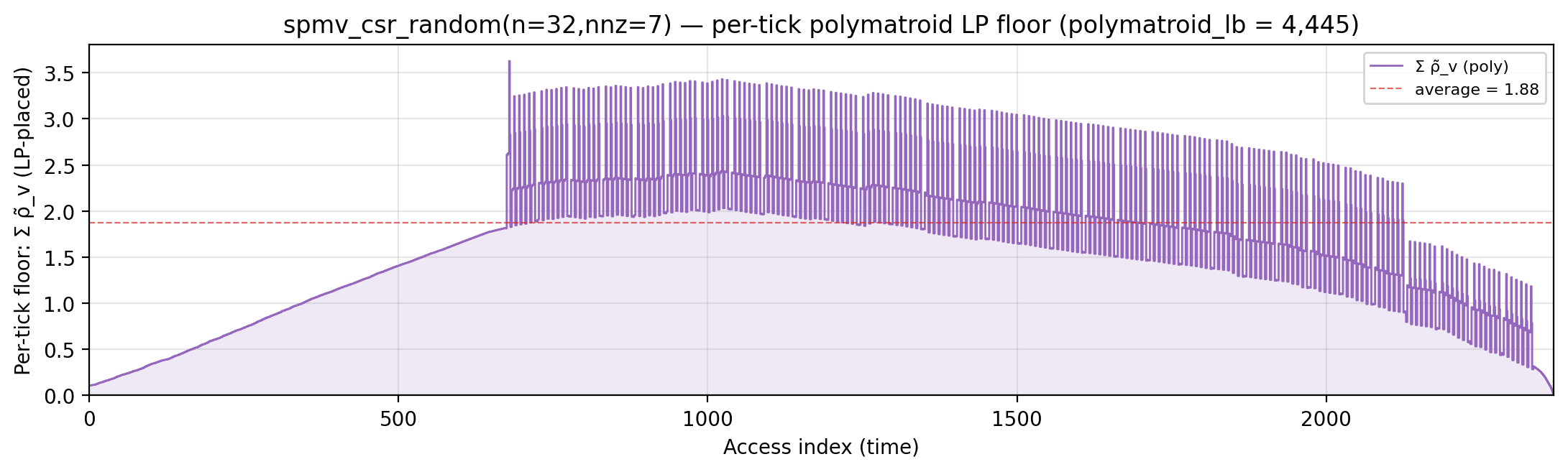
Rolling spatial intensity — heartbeat plot of ops / Σ ⌈√d⌉ over a sliding window.
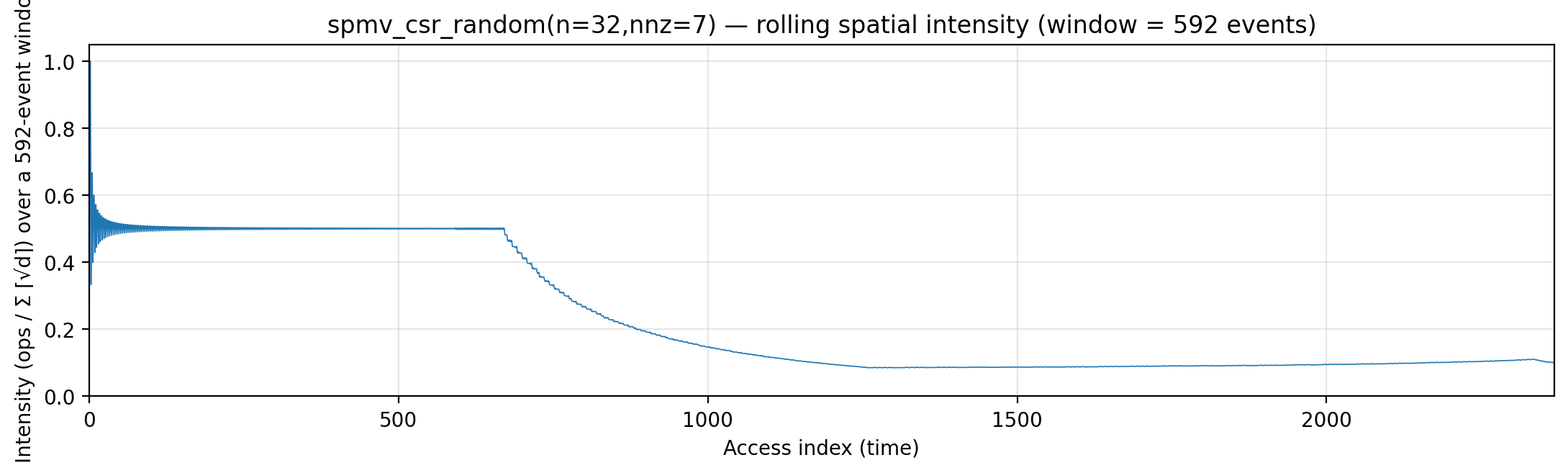
Cumulative compute vs fetch cost — slope = instantaneous spatial arithmetic intensity.
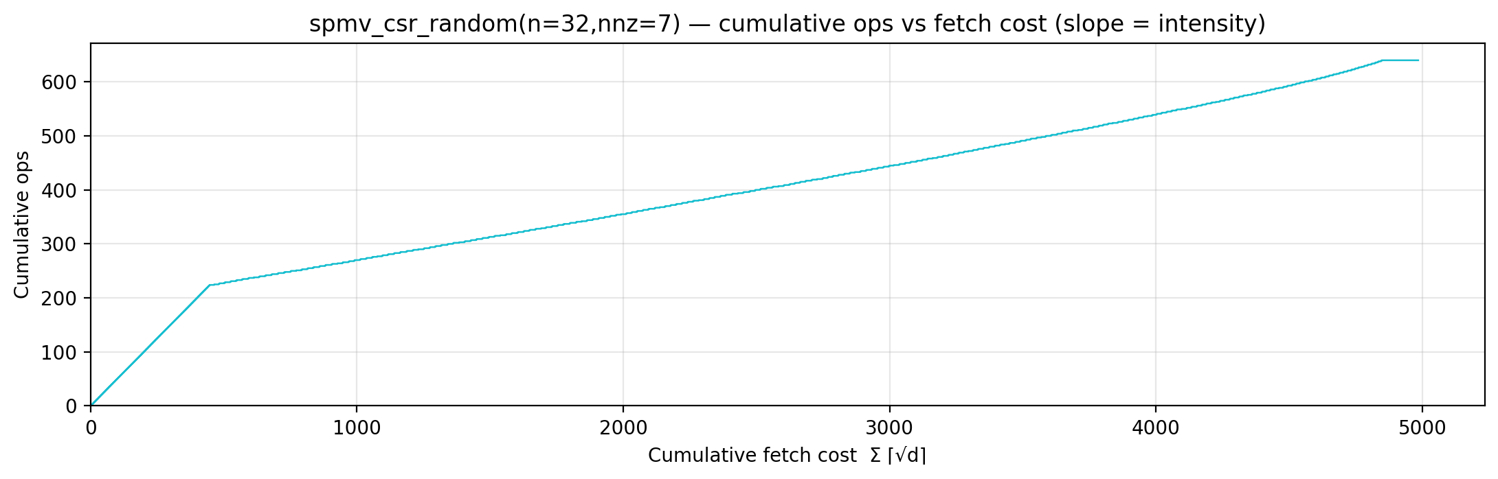
Gravity well — per-load fetch-cost ⌈√d⌉ scatter.
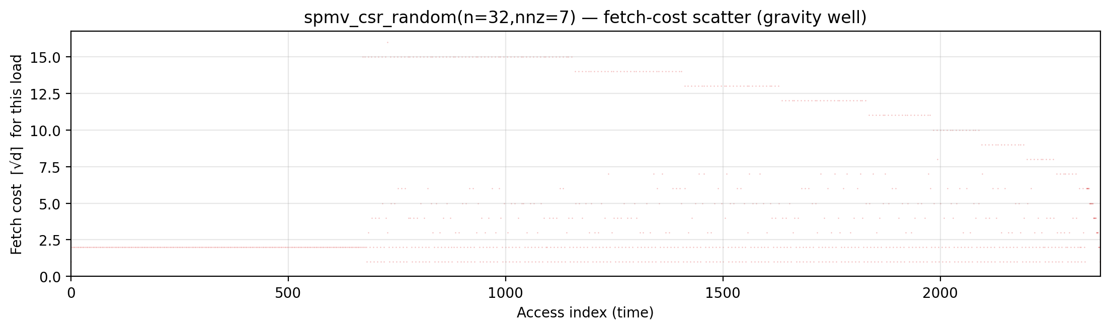
Spatial locality CDF — compute-fulfillment as a function of radius.
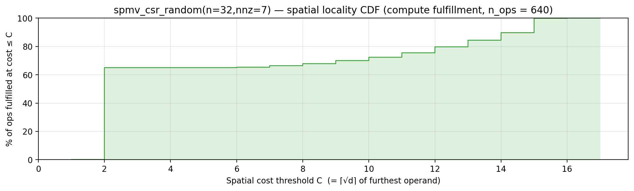
Working-set size over a τ = 163-event window (max = 96).
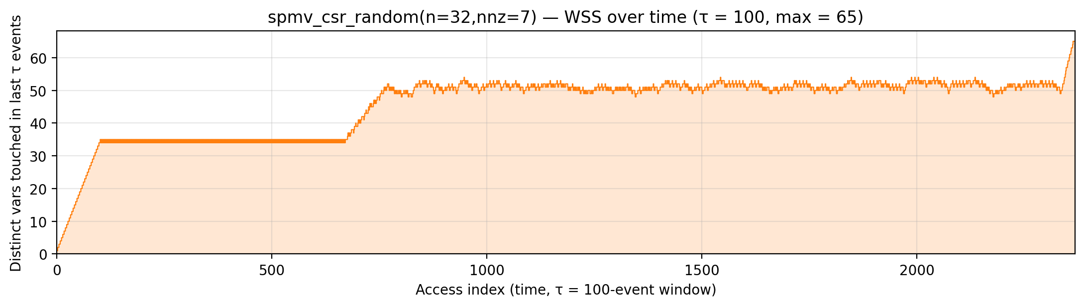
bitonic_sort (code)
N=64. Algorithm. Data-oblivious sorting network: log²N compare-swap passes in butterfly order (identical in flavor to the iterative FFT).
Manual. Input preloaded to scratch; every pass does N/2 pair compare-swaps against varying-stride partners, exercising the full scratch range uniformly.
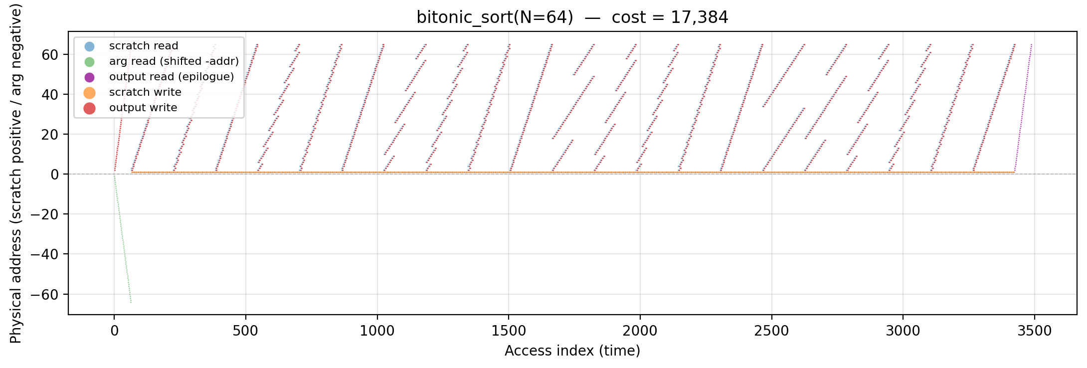
Working-set size over time (peak = 64).
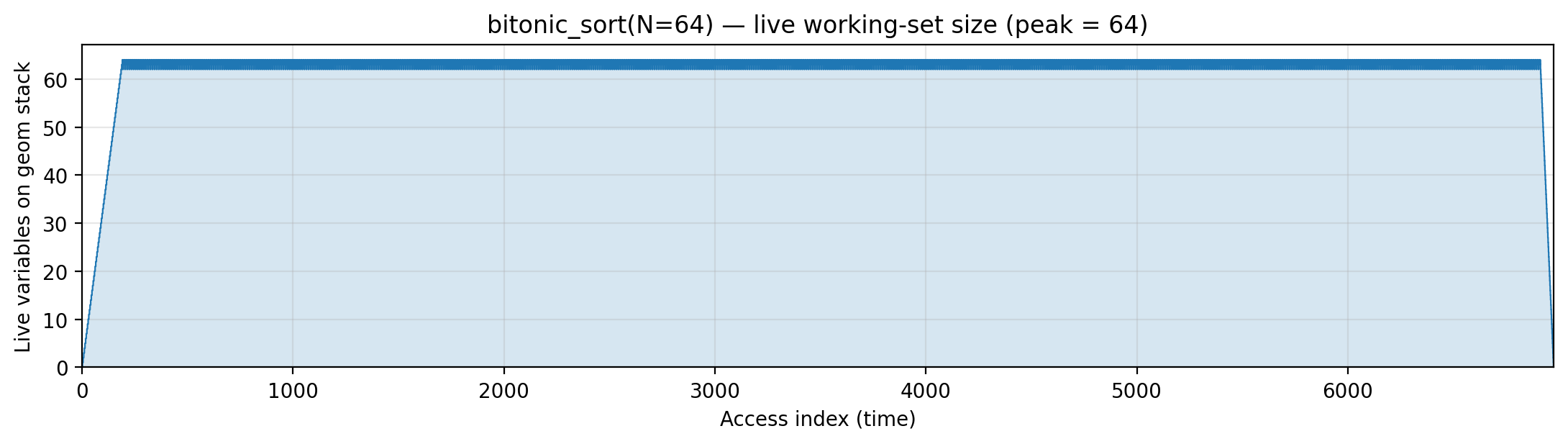
Reuse distance per load — LRU vs Bélády OPT (max LRU = 64; max OPT = 64).
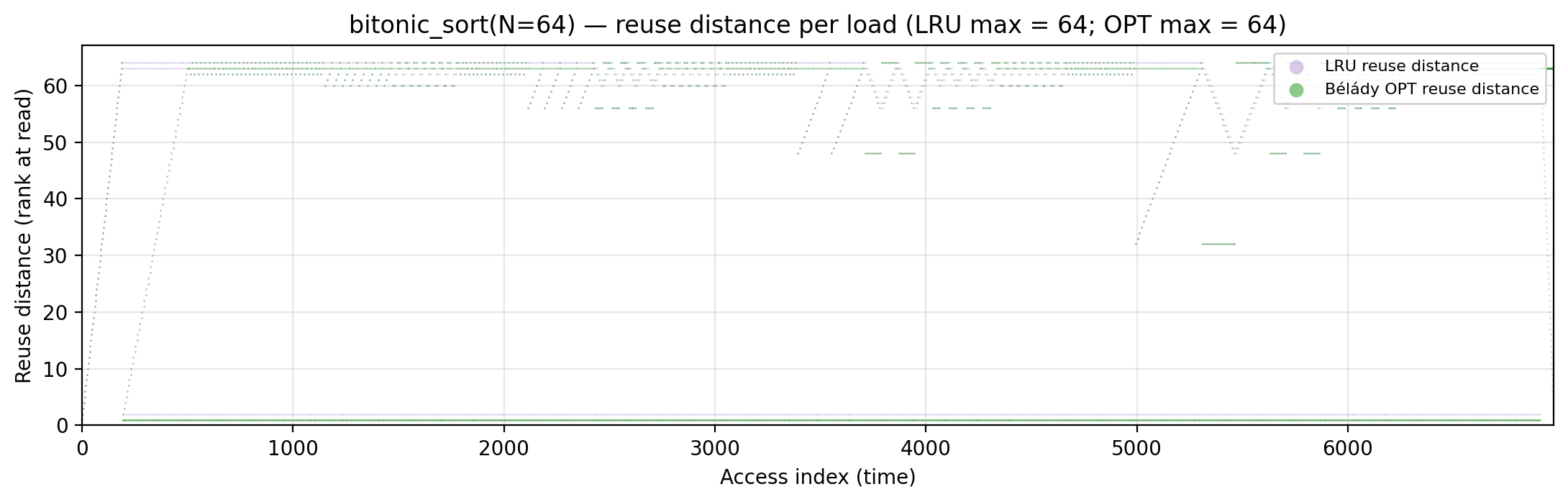
Miss-ratio curve — LRU vs Bélády OPT misses by cache capacity.
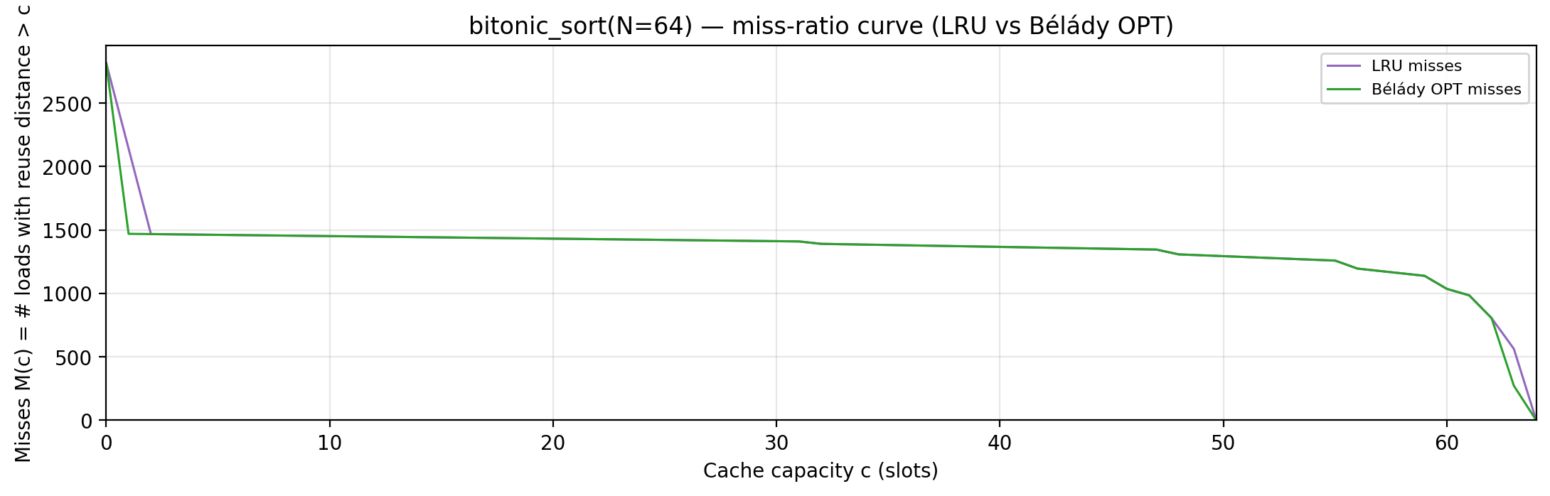
Per-tick TU LP floor — integrand of global_density: Σ_i ρ_{(i)} · √i over currently-live vars, ranked by density; the area equals global_density.
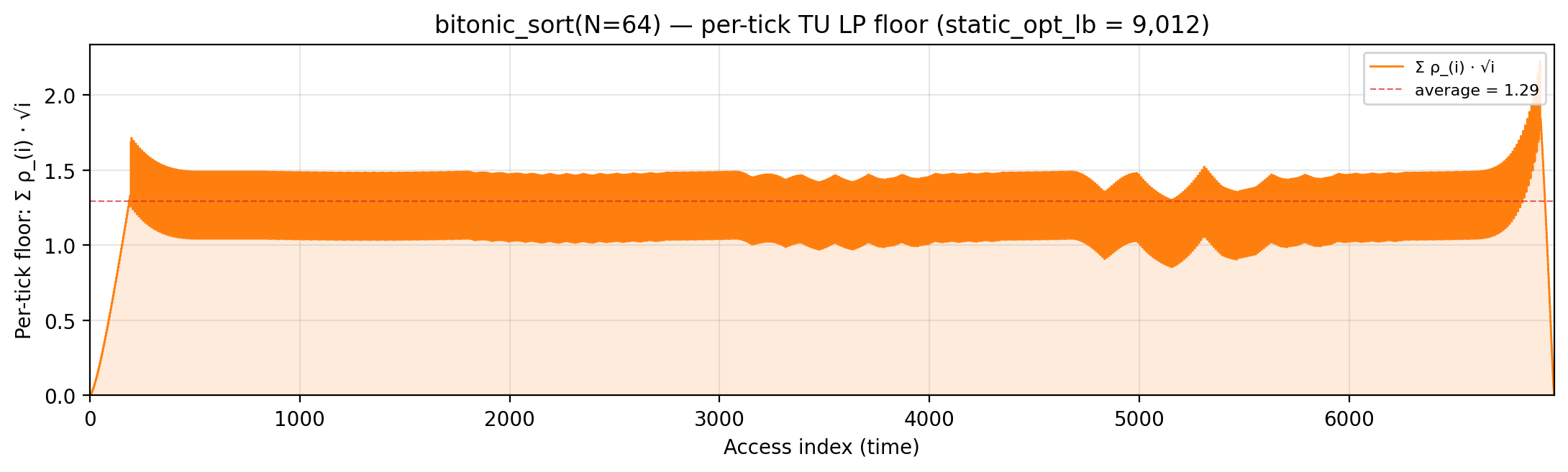
Per-tick splitting LP floor — integrand of local_density: Σ_i ρ_{(i)} · √i over the currently-active per-burst virtual intervals; the area equals the geometric portion of local_density.

Per-tick polymatroid LP floor — integrand of polymatroid_lb: Σ_v reads_v · ⌈√d_v⌉ / lifespan(v) over live vars, where d_v is each variable’s LP-implied static depth (gemini/polymatroid-relaxation.md). The area equals the geometric portion of polymatroid_lb.

Rolling spatial intensity — heartbeat plot of ops / Σ ⌈√d⌉ over a sliding window.
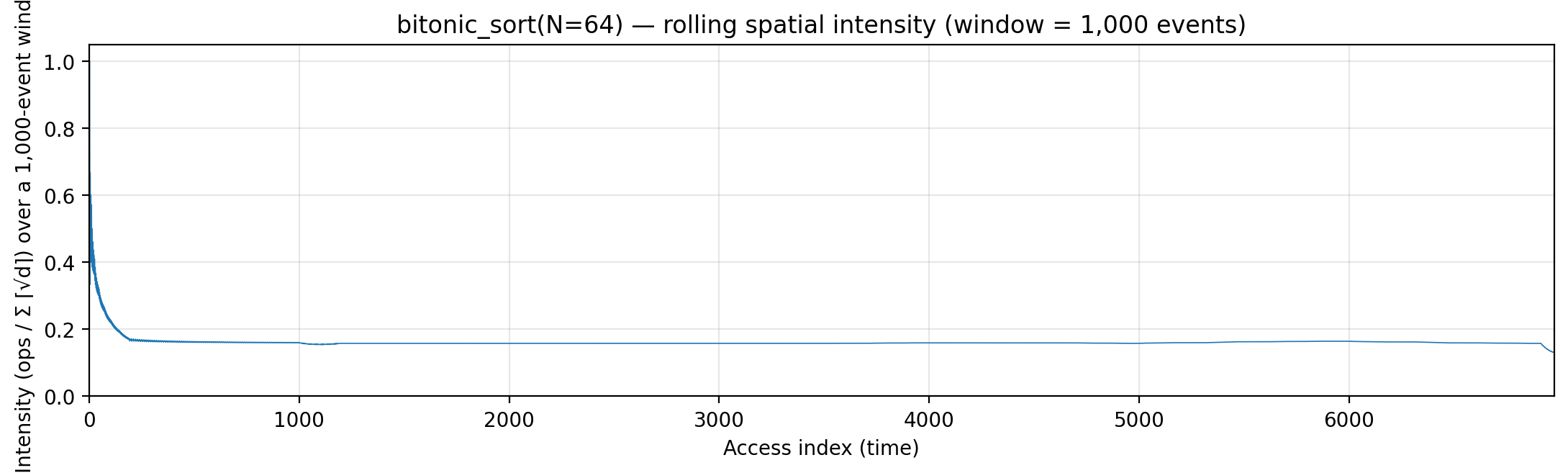
Cumulative compute vs fetch cost — slope = instantaneous spatial arithmetic intensity.
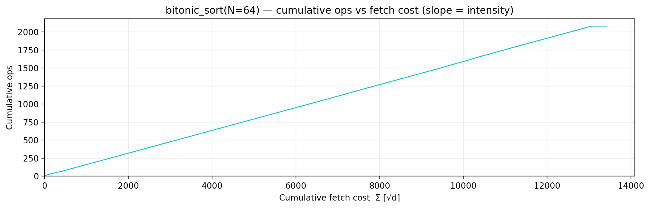
Gravity well — per-load fetch-cost ⌈√d⌉ scatter.
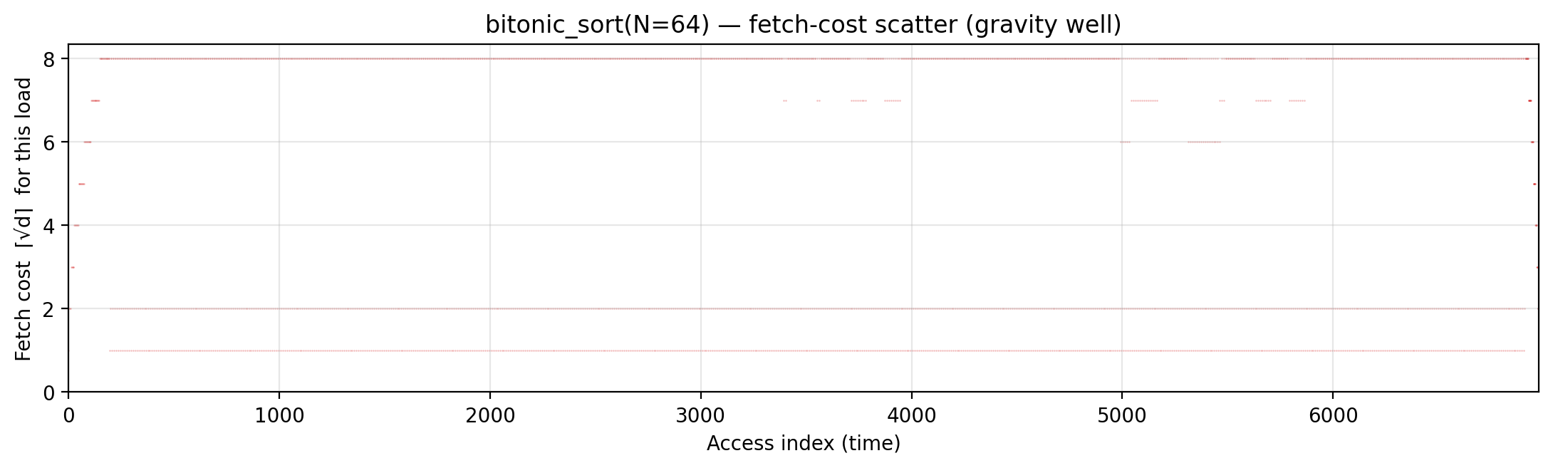
Spatial locality CDF — compute-fulfillment as a function of radius.
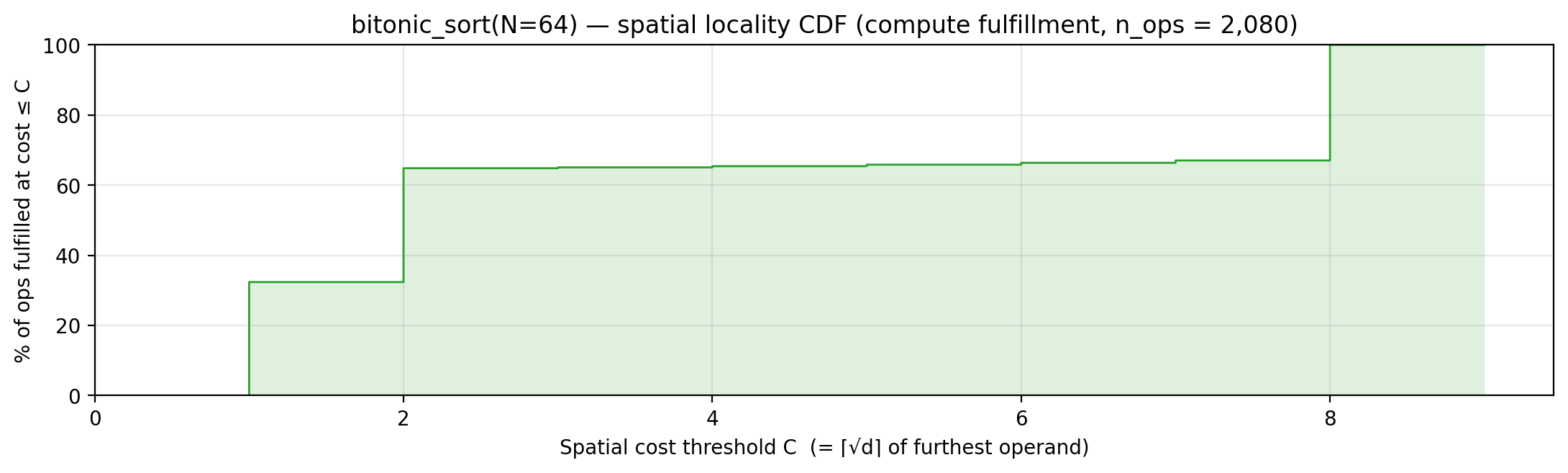
Working-set size over a τ = 64-event window (max = 64).