Backprop versus
the memory wall.

0. Summary

The unit. Your unit is exactly Dally's 2023 unit: an add costs about 1 fJ/bit and on-chip wire about 100 fJ/bit·mm, so one add is worth 10 µm of movement and one bit across a 16 mm die is worth 1,600 adds. In that unit, on an A100: a byte from HBM costs ~5,000 adds at the memory interface and ~7,500 all-in (add the on-die round trip); a byte from the 40 MB L2 ~1,500; a byte from shared memory ~120; and a BF16 FLOP costs ~12 adds in the datapath but ~110 adds all-in, because the other ~100 are operand delivery and orchestration. Arithmetic is the cheapest thing a training step does.

Eleven heuristics (all derived below; numbers are A100-80GB unless stated):

1. Reuse rule. A byte fetched across boundary $i$ must be reused at least $\beta_i$ times, where $\beta_t = \text{peak}/\text{bandwidth}$ (time) and $\beta_E = e_\text{byte}/e_\text{FLOP}$ (energy). At HBM: $\beta_t = 153$ FLOP/B, $\beta_E = 67$ (A100); $295 / 91$ (H100). $\beta_t$ roughly doubles per GPU generation while on-chip capacities do not, so tiles and batches must keep growing.
2. Training-step intensity. At the HBM boundary, $I(T) \approx \dfrac{72\,T d}{12\,b_w d + a\,T}$: it is $\approx T/2$ while weights are being streamed and saturates at $\approx 72d/a \approx 0.36\,d$ (about $10^3$ FLOP/B at $d = 4096$ once L2 re-blocking is included).
3. Batch floor. $T_{\min} = \dfrac{12\,b_w d\,\beta_t}{72 d - a\,\beta_t} \to 2\beta_t \approx 300$ tokens per weight visit on A100, $\approx 600$ on H100, diverging at $d_{\min} = a\beta_t/72 \approx 450$ (A100) / $900$ (H100). Below $d_{\min}$ no batch size helps; only fusion does.
4. Rank rule. A micro-batch of $T$ tokens carries at most rank-$T$ information per weight matrix. Moving $W$ or $\nabla W$ ($dk$ numbers) instead of the factors $X, \nabla Y$ ($T(d+k)$ numbers) is redundant while $T < dk/(d+k) \approx 0.8\,d$. The same "$T \approx d$" threshold falls out from the information side as from the bandwidth side.
5. Element-wise time tax $\approx a\beta_t/(72d) \approx 2.8\,\beta_t/d$ of GEMM time: 10% at $d = 4096$, 55% at $d = 768$ on A100, 107% at $d = 768$ on H100. The corresponding energy tax is only $a\,e_B/(72\,d\,e_F) \approx 4.5\%$ at $d = 4096$. Backprop's activation round trip is cheap in joules and expensive in seconds.
6. Store versus recompute. Round-tripping a token-layer's saved activations through HBM costs $68\,d\,e_B$; recomputing the forward costs $24\,d^2 e_F$. Storing wins for $d > 2.8\,e_B/e_F \approx 190$. Gradient checkpointing therefore buys capacity at +33% arithmetic energy; it lowers no traffic.
7. Per-step fixed traffic. Adam in mixed precision moves ~30 B/param/step: parity with compute at $T_\text{step} \approx 5\beta_t \approx 800$ tokens per device, <10% overhead at ~$10^4$. Data-parallel ring all-reduce moves ~4 B/param over the fabric: $T_\text{dev} \ge \beta_\text{net}/1.5 \approx 700$ (NVLink) or $\approx 8{,}000$ (IB HDR) per step. ZeRO-3/FSDP moves ~6 B/param per micro-batch: $T_\text{dev} \ge \beta_\text{net}$ per micro-batch.
8. Model-parallel escape. Tensor parallelism's fabric intensity is $4.5\,d/p$ FLOP/B and pipeline parallelism's is $18dL/p$; both are batch-independent. Only data parallelism's is $\propto T$.
9. The squeeze. With McCandlish's $S = S_{\min}(1 + B_\text{crit}/B)$ and a fixed per-step cost worth $T_\text{fixed}$ token-equivalents per device, the time-optimal global batch is $B_\text{opt} = \sqrt{B_\text{crit}\, N\, T_\text{fixed}}$, the geometric mean of the statistical ceiling and the hardware floor. At $N = 1024$ over IB the optimum sits inside the communication wall ($T_\text{dev} \approx 2{,}800 <$ parity at $8{,}300$).
10. On the grid. For a weight-stationary layer on $n$ tiles, hops per FLOP $= (d+k)\sqrt n/(dk)$ byte-hops, independent of batch; the backward pass is the forward pass with flow reversed (the transpose is free) and $\nabla W$ is a local outer product. What backprop costs spatially is in-flight storage $\propto L \times (\text{pipeline stages})$, i.e. $L^2$ when fully spatial, versus $L$ for forward-only. That $L^2$ is the wall backprop hits on a Dally grid; reversible layers delete it for +33% FLOPs.
11. Single example. Online per-token backprop of a 7B model on an A100 runs ~1,000× below the roofline: 25 J and 140 ms per token, 0.1% of the energy in arithmetic. Single-sequence backprop (2,048 tokens) is only 1.5× off on one GPU (the sequence is the batch), but 5× off across 64 GPUs over IB. Sixty-four sequences per GPU bring it to 1.16× and ~50 mJ/token.

1. Compute versus commute

Definitions. For any kernel or algorithm and any boundary (register file, shared memory, L2, HBM, NVLink, InfiniBand, or a hop on a spatial grid):

• operational intensity $I$ = FLOPs per byte crossing the boundary (Williams, Waterman & Patterson 2009);
• machine balance $\beta_t$ = peak FLOP/s ÷ bandwidth across it, and energy balance $\beta_E$ = $e_\text{byte}/e_\text{FLOP}$;
• compute-to-commute ratio $\chi = I/\beta$; behind the wall when $\chi < 1$;
• time slowdown $= \max(1, \beta_t/I)$; commute share of energy $= \beta_E/(I + \beta_E)$.

Table 1 — the price list (A100-class, 7 nm; estimates, sources in appendix).

Table 2 — balances at the HBM boundary.

Two things this table says that are easy to miss:

• $\beta_E < \beta_t$ on every GPU. A kernel that just reaches the roofline knee ($I = \beta_t$) still spends $\beta_E/(\beta_t + \beta_E) \approx 30\%$ of its energy on HBM bytes on A100. Time-balance and energy-balance are different targets; the energy target is easier, which is why memory-bound kernels are worse in seconds than in joules.
• The FLOP price is itself mostly commute. The all-in 0.9 pJ/FLOP is ~9× the datapath. It is set by tile-level reuse and by physical distance to L2, not by batch. For an $M \times N$ output tile the shared-memory intensity is $MN/(M+N)$ FLOP/B: 64 for 128×128, 85 for 256×128, against $\beta_\text{SMEM} \approx 16$ and $\beta_\text{L2} \approx 60$ on A100. Hopper's L2 balance sits at or above that tile intensity, which is why it needed 4–8× larger tiles (wgmma, TMA, clusters). This is the interior memory wall and no batch size touches it; only bigger tiles, fewer bits, or a spatial dataflow do.

2. The ledger of one training step

Per GPT-style layer with a $4d$ FFN: $P_\ell = 12d^2$ parameters; arithmetic $F = 72\,d^2$ FLOPs per token (forward $24d^2$, backward $48d^2$) plus $\approx 12\,s\,d$ for attention at sequence length $s$ (forward $4sd$, backward $\approx 8sd$ with FlashAttention's recompute), which is 8% of the total at $s = 2048$, $d = 4096$ and is included in the recipe.

Bytes crossing the HBM boundary, per layer:

Putting (a), (b), (d) together, the HBM intensity of one layer's forward + backward as a function of tokens per weight visit $T$ is

The first branch is the weight-streaming regime (every byte of $W$ is used $T$ times, twice), the second the activation regime (traffic $\propto T$, intensity saturates). The crossover between them is at $T \approx 12\,b_w d/a \approx 0.7\,d$: the batch at which the bytes spent on activations equal the bytes spent on weights. That is the bandwidth-side version of the rank rule (heuristic 4).

3. Intensity versus batch: three floors and one ceiling

(a) Training-step intensity vs. batch(b) Batch needed to leave the HBM wall(c) Where the joules go

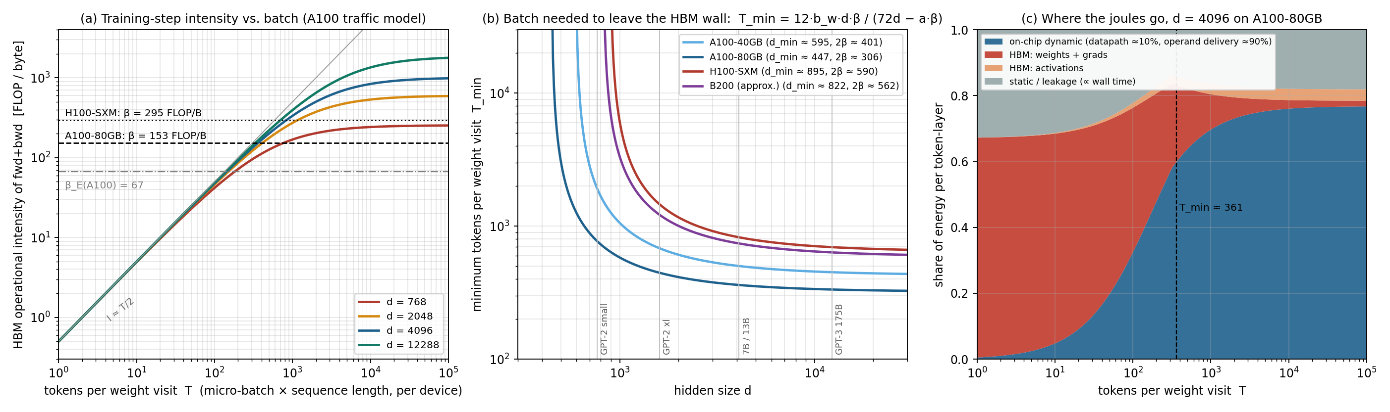
Floor 1 — weight reuse at HBM (per micro-batch, per weight-holding device). Solving $I(T) \ge \beta_t$:

Table 3 — tokens per weight visit needed to reach $\beta_t$.

Three remarks. First, "tokens per weight visit" is the micro-batch on one device, in tokens: with gradient accumulation the weights are re-streamed every micro-batch, so $T$ is micro-batch × sequence length, not the global batch. Tensor parallelism leaves $T_{\min}$ unchanged (per-device FLOPs and per-device weight bytes shrink together). Second, for any $d \ge 1024$ a single 2,048-token sequence already satisfies this floor on A100 and H100: the sequence is the batch, which is the transformer's great advantage over an MLP on vectors, where $T$ = the example count. Third, the floor is generation-dependent in the wrong direction: H100 needs 2.3× the tokens A100 does at $d = 4096$, and its $d_{\min}$ has moved above GPT-2-medium.

Floor 2 — the small-$d$ pole. $T_{\min}$ diverges at $d_{\min} = a\beta_t / 72$ (447 on A100-80GB, 895 on H100). Below it the inter-kernel activation traffic alone exceeds the balance and no batch size exits the wall, because that traffic is proportional to $T$. The only levers are $a$ (fusion, FP8 storage) and the ratio $\beta_t$ (a slower, cheaper part). This is why GPT-2-small-sized models get 20–30% MFU on H100 no matter how they are batched.

Floor 3 — per-step fixed traffic. Terms (e) and (f) are paid once per optimizer step, not per micro-batch:

with $\beta_\text{net} = \text{peak}/\text{per-direction fabric bandwidth}$: 1,040 FLOP/B for NVLink-3 (300 GB/s per direction), 12,500 for one HDR NIC (25 GB/s). The last two rows are the escape hatch: tensor and pipeline parallelism add devices without adding batch, because their communication scales with $d$, not $T$. Data parallelism is the only axis whose communication demands batch, which is why the batch-size question is really a data-parallel-width question.

The ceiling — critical batch size. Beyond the gradient-noise scale, batch stops buying steps: McCandlish et al. 2018 give $S = S_{\min}(1 + B_\text{noise}/B)$ steps and $E = E_{\min}(1 + B/B_\text{noise})$ tokens; Kaplan et al. 2020 fit $B_\text{crit}(L) = B^*/L^{1/\alpha_B}$ with $B^* \approx 2 \times 10^8$ tokens and $\alpha_B \approx 0.21$, i.e. $B_\text{crit} \approx 0.5$–$4 \times 10^6$ tokens at the losses where pre-training lives (production runs use 2–16 M). So the memory-wall-free window is roughly

about two orders of magnitude wide for a 7B model on a few hundred GPUs, and it closes as $N$ grows or $d$ shrinks.

The squeeze. Put the fixed cost and the ceiling in one objective. Per-device step time is $t = 6P\,T_\text{dev}/\text{peak} + t_\text{fixed}$; write $T_\text{fixed} = t_\text{fixed}\,\text{peak}/6P$ (the fixed cost in token-equivalents) and $B = N T_\text{dev}$. Total time $S(B)\,t(B)$ is minimized at

Table 4 — the squeeze for a 7B model, $B_\text{crit} = 10^6$, no communication overlap.

At 1,024 GPUs over InfiniBand the time-optimal per-device batch (2,849 tokens) is below the communication-parity point (8,313): the optimizer deliberately operates inside the wall because the alternative, pushing $B$ past $B_\text{crit}$, wastes samples faster than the wall wastes seconds. This is a sub-optimization result in your sense: a hardware team maximizing MFU and a research team maximizing sample efficiency pull toward different $B$, and the joint optimum is the geometric mean of their two targets. Overlap (the usual fix) reduces $T_\text{fixed}$ but does not change the form.

4. What is specifically backprop's fault

(a) Weight-side: not much. The backward pass reads $W$ once more for $\nabla X$ and reads $X$ and $\nabla Y$ for $\nabla W$; it triples the FLOPs and roughly doubles the bytes, so per pass its intensity is the same $T$ FLOP/B as the forward pass. Backprop does not make the matmuls memory-bound. Its weight-side floor is twice that of inference decode only because of the fp32 gradient read-modify-write (the "12" in $b_w$), which is a choice of numerics, not of algorithm; with bf16 gradients the floor is $\beta_t$, identical to decode.

(b) Temporal non-locality: the real thing. The forward activation of layer $\ell$ is produced at time $t_\ell$ and consumed at $t_{2L-\ell}$. On a time-multiplexed machine that is a capacity cost of $34\,d \cdot T \cdot L$ bytes per micro-batch (9.1 GB per 2,048-token sequence for a 32-layer $d = 4096$ model; 73 GB for eight of them, which is why eight sequences become eight micro-batches and $T$ per weight visit stays 2,048), and it is what checkpointing and reversibility address. On a spatial machine it is an in-flight cost, Section 6.

(c) The store-versus-recompute energetics. Storing and reloading a token-layer's activations costs $2 \times 34\,d \times e_B = 4.1\,d$ nJ; recomputing the forward costs $24\,d^2 \times e_F = 21.6\,d^2$ pJ. They cross at $d \approx 190$; above it storing is cheaper. Full checkpointing (store only the $2d$ layer input, recompute the rest) therefore costs +33% arithmetic energy for a 17× capacity reduction, and lowers HBM traffic not at all; selective recompute (Korthikanti's attention-only variant) gets most of the capacity at ~3% arithmetic. FlashAttention is the case where recompute wins on traffic: the $s \times s$ score matrix has O(1) intensity through HBM, so recomputing it in shared memory during the backward pass ($\approx 4sd$ extra FLOPs per token) removes $O(s^2)$ bytes.

(d) The rank-$T$ argument. $\nabla W = X^\top \nabla Y$ has rank $\le T$. A micro-batch's update to a $d \times k$ matrix contains at most $T(d+k)$ independent numbers, yet a time-multiplexed implementation moves $dk$ numbers of $W$ (twice) and $dk$ numbers of $\nabla W$ (read-modify-write) to apply it. The bytes are $dk/(T(d+k)) \approx 0.8\,d/T$ times redundant. At $T = 1$ and $d = 4096$ that is a 3,300× overhead in bytes per unit of information, which is the entire per-token memory wall stated without reference to any bandwidth number. Weight-stationary arrays, LoRA-style factored updates and GaLore all exploit the same fact; the factors are cheaper to move than the product until $T \approx d$.

(e) The time tax and why fusion, not batch. The inter-kernel traffic $a\,d$ per token is $T$-proportional, so it is a fixed fraction of step time, $a\beta_t/72d$, regardless of batch: 10% at $d = 4096$ and 55% at $d = 768$ on A100 (twice that on H100). During those seconds the tensor cores idle but the leakage clock runs, which is the ~20% static slice in Figure (c). Batching cannot shrink this slice; kernel fusion, FP8 activation storage, and reversibility can.

5. Single-example backprop, quantified

Table 5 — 7B-class model ($d = 4096$, $L = 32$, $s = 2048$, 6.85 B params) on A100-80GB; no communication overlap; GEMMs at peak (multiply the arithmetic time by 1/MFU for a real stack). Tokens per step are per GPU.

Your intuition is right in the limit and needs one refinement in the middle:

• Per token (online learning, RL with per-step updates, streaming): catastrophic. Every layer streams 2.4 GB of weights and gradient state for 1.2 GFLOP of work; the step is 1,000× slower than compute-bound and 500× more energy per token than the batched regime. Nothing about this improves with the GPU generation, because $\beta_t$ grows.
• Per sequence, one GPU: the sequence supplies ~2,000 tokens of weight reuse, so the GEMMs sit above $\beta_t$ ($I = 237$). What is left is the per-step fixed traffic (205 GB of optimizer state per step against 0.27 s of compute), a 1.46× slowdown and ~60 mJ/token. Note also that Adam's state alone (110 GB) does not fit, so single-sequence training of a 7B model on one A100 is a capacity problem before it is a bandwidth one.
• Per sequence, many GPUs: the DP all-reduce of 27 GB of gradients per step over a 25 GB/s NIC costs 1.1 s against 0.27 s of compute: 5× slowdown, half the energy is leakage while waiting. This is the regime in which "single example backprop is inefficient" is most true in practice, and it is a fabric wall, not an HBM wall.
• Batched: 8 sequences per GPU recover to 1.6×, 64 to 1.16×; the remaining 16% is the element-wise time tax plus the ~10% per-step terms. Energy floors at ~50 mJ/token with 73% in on-chip dynamic power, of which roughly a tenth is the actual multiply-adds.

For contrast: a CNN gets its reuse from spatial positions (a 224² image supplies ~50k positions per convolution weight) and is fine at batch 1; an MLP on vectors is the worst case, with $T$ equal to the example count; decode-time inference is the transformer's own worst case, because the KV cache is per-sequence and batching does not amortize it. Dally's Megatron-20B slide shows exactly that: a hypothetical Hopper with 10× the HBM bandwidth is still 3.6× faster at batch 256, so even large-batch decode remains bandwidth-bound.

6. On Dally's grid

I could not fetch your repository (GitHub refuses automated access), so I use the model your directory name points to: the spatial computer of Gianinazzi, Ben-Nun, Besta, Ashkboos, Baumann, Luczynski & Hoefler (2022), in which processors sit on a 2D grid, the energy of a computation is the total byte-distance travelled by all messages, and the depth is the longest chain of hops; a variant adds a local-memory size parameter. Map "hop" to your model's unit; the ratios below do not depend on it.

Forward pass. Put a $d \times k$ layer, weight-stationary, on a $\sqrt n \times \sqrt n$ block of tiles, each holding a $(d/\sqrt n) \times (k/\sqrt n)$ slice. Per token, the $2d$ input bytes travel across a row of $\sqrt n$ blocks and the $2k$ output bytes (partial sums) travel down a column of $\sqrt n$ blocks: $2(d+k)\sqrt n$ byte-hops for $2dk$ FLOPs, i.e.

For $d = 4096$, $k = 16384$ on $n = 256$ tiles (0.5 MB of weights each): $4.9 \times 10^{-3}$ byte-hops per FLOP, which at 0.5 mm pitch (0.4 pJ per byte-hop, 50 adds) is 0.002 pJ/FLOP, 2% of the datapath. Spatially the matmul is not the problem, and this is batch-independent: hops per FLOP depend on array geometry, not on $T$.

Backward pass. $\nabla X = \nabla Y\, W^\top$ is the same array with the flow reversed: $\nabla Y$ enters where $Y$ left, partial sums exit where $X$ entered. The transpose costs zero hops; that is the single biggest structural advantage a spatial layout has over a time-multiplexed one for backprop. $\nabla W = X^\top \nabla Y$ is an outer product, and each tile already sees exactly the slices of $X$ and $\nabla Y$ it needs pass through it. So $\nabla W$ costs no hops if each tile remembers its slice of $X$ until $\nabla Y$ arrives: storage of $T \cdot d/\sqrt n$ elements per tile, i.e. the layer input replicated $\sqrt n$ times across the column blocks. The alternative, storing $X$ once at the layer boundary and re-broadcasting it when $\nabla Y$ comes back, costs a second $2d\sqrt n$ byte-hops per token. Either way the backward pass pays a $\sqrt n$ factor that the forward pass did not, in storage or in hops.

In-flight storage: the $L^2$. A token that passes layer $\ell$ at time $\ell\tau$ returns to it at $(2L-\ell)\tau$. With the pipeline full, the tokens layer $\ell$ must hold number $2(L-\ell)$ times the tokens admitted per layer-latency, so the total in-flight activation storage is

where $T_\tau$ is the tokens in flight per layer. On a GPU pipeline with $p \ll L$ stages the same sum gives $\tfrac12 L p\, T_\tau\, c\, d$ (the 1F1B schedule of GPipe/PipeDream); a fully spatial machine is $p = L$. For $L = 32$, $d = 4096$, $T_\tau = 256$: 37 GB store-all, 2.1 GB inputs-only, versus 4.6 GB for the same model on an 8-stage GPU pipeline. Forward-only inference and any local learning rule have $L$, not $L^2$. This quadratic in depth, not the matmul hops, is the memory wall backprop hits on a Dally grid, and it is why wafer-scale designs invert the mapping (Cerebras streams weights past resident activations one layer at a time, which removes the $L^2$ and reinstates the "batch ≥ $\beta$ of the weight fabric" rule instead).

Batch on the grid. Since hops per FLOP are batch-independent, batch matters on the grid only through local weight reuse: reading a weight from a tile's SRAM costs ~1 pJ/byte, 5–10× a MAC, so weights must be held in registers and applied to $T_\text{local} \ge e_\text{SRAM}/e_\text{MAC} \approx 10$ inputs before being refetched. This is the TPU's weight-stationary systolic dataflow, and it is the same reuse rule as heuristic 1 with $\beta_\text{SRAM} \approx 10$ instead of $\beta_\text{HBM} \approx 150$. The grid converts a batch problem into a register-file problem.

What to count. For a hop-counting comparison of algorithms on the grid, four quantities capture the above: forward byte-hops, backward byte-hops (including any $X$ re-broadcast), the in-flight byte-seconds $\sum_\ell 2(L-\ell)\,\tau\,(\text{bytes stored at } \ell)$, and the depth $2L\sqrt n$. Backprop's signature is a factor ~2 on the first two, $\sqrt n$ on the second, and $L$ on the third relative to the forward pass.

7. What "solving it at prescribed accuracy" would take

The analysis says the wall has three separable parts, and existing proposals each attack one:

The honest summary for your problem statement: with backprop kept exact, the wall is already beatable in bandwidth and energy terms for $d \gtrsim 1000$ by (i) $T \ge$ a few hundred tokens per weight visit, which a single sequence supplies, (ii) fusion and low-precision storage for the $a\,d$ term, (iii) model parallelism to add devices without adding batch, and (iv) reversibility or recompute for capacity. What no exact method removes is the per-step fixed traffic (which is why the squeeze exists) and the interior wall inside the FLOP. The approximate methods that remove the $L^2$ outright have not yet met "prescribed accuracy" at scale; the cleanest candidate that is both exact and spatially local is the reversible network, which turns backprop into a second, backwards forward pass and makes every layer's storage O(1) in depth.

8. Measuring it

On the A100 with NVML. Use nvmlDeviceGetTotalEnergyConsumption (a millijoule counter, Volta and later), not nvmlDeviceGetPowerUsage: the power reading on A100 is a windowed average that undersamples kernels shorter than a few hundred milliseconds, so repeat each kernel for ≥ 1 s and difference the counter. Two calibration kernels give you the constants of this report directly:

• a bandwidth-bound kernel (a large element-wise op or a device-to-device copy, ~2 TB/s): $(P_\text{kernel} - P_\text{idle}) / \text{bytes per second}$ is the all-in HBM energy per byte; the model predicts ~120 W above idle, i.e. ~60 pJ/B, and any gap from the 40 pJ/B interface figure is the on-die transport you have been trying to reconcile with Dally's wire numbers;
• a large BF16 GEMM at ~290 TFLOP/s: $(P - P_\text{idle} - P_\text{HBM})/\text{FLOP/s}$ is the all-in energy per FLOP, predicted ~0.9 pJ.

The signature to look for in a training step is bimodal power: ~380–400 W during GEMMs, ~200–250 W during the element-wise and optimizer phases. The fraction of time in the low mode is the time tax of heuristic 5; the energy in it is the static slice of Figure (c).

On the grid. Count separately the four quantities of Section 6 and report backprop as ratios to the forward pass: byte-hops (expect ~2×, plus the $\sqrt n$ re-broadcast if you choose not to replicate $X$), in-flight byte-seconds (expect ~$L$×), and depth (2×). A candidate algorithm "solves the problem" in the sense of your prompt if it brings the in-flight term from $L^2$ to $L$ without raising the byte-hop term by more than the +33% that reversibility costs in arithmetic.

Appendix — parameters and their provenance

References. Dally, Energy Efficiency and AI Hardware, Stanford AHA retreat, 2023; Dally, "On the model of computation: point", CACM 65(9), 2022; Williams, Waterman & Patterson, "Roofline", CACM 2009; Hong & Kung, "I/O complexity: the red-blue pebble game", STOC 1981; Korthikanti et al., "Reducing activation recomputation in large transformer models", 2022; Dao et al., "FlashAttention", 2022; Chen et al., "Training deep nets with sublinear memory cost", 2016; Griewank & Walther, "Algorithm 799: revolve", 2000; Gomez et al., "The reversible residual network", 2017; Huang et al., "GPipe", 2019; Narayanan et al., "PipeDream", 2019; Rajbhandari et al., "ZeRO", 2020; McCandlish et al., "An empirical model of large-batch training", 2018; Kaplan et al., "Scaling laws for neural language models", 2020; Gianinazzi et al., "The spatial computer", 2022; Jouppi et al., "In-datacenter performance analysis of a TPU", 2017; Jaderberg et al., "Decoupled neural interfaces using synthetic gradients", 2017; Nøkland & Eidnes, "Training neural networks with local error signals", 2019; Belilovsky et al., "Greedy layerwise learning can scale to ImageNet", 2019; Hinton, "The forward-forward algorithm", 2022; Baydin et al., "Gradients without backpropagation", 2022; Ren et al., "Scaling forward gradient with local losses", 2023; Malladi et al., "Fine-tuning language models with just forward passes", 2023.