AIR Multi-MNIST (Attend, Infer, Repeat)
Numpy reproduction of Eslami, Heess, Weber, Tassa, Szepesvari, Kavukcuoglu & Hinton, “Attend, Infer, Repeat: Fast Scene Understanding with Generative Models”, NIPS 2016. The paper’s headline claim: a recurrent attention model can simultaneously learn to count, locate, and identify a variable number of objects in a scene with no per-object supervision – only the raw scene as the reconstruction target.
Problem
A 32x32 canvas containing 0, 1, or 2 randomly placed and scaled MNIST digits (scale 12-18 pixels, uniformly random position within bounds). Each scene is labelled only with the raw pixel image – no per-digit boxes, no count label. The model must infer:
- Count: how many digits are present (0, 1, or 2).
- Location: a 3-D affine
(scale, dx, dy)per digit. - Appearance: a low-dimensional
z_whatlatent per digit.
Chance for the count is 1/3 ≈ 0.333 (uniform over {0, 1, 2}); the spec
target for “best-effort numpy” is count_acc > 0.5.
Architecture
| Stage | Layer | Output shape | Notes |
|---|---|---|---|
| Input | – | (B, 32, 32) | scene |
| Encoder fc1 | 1024 -> 200, ReLU | (B, 200) | global MLP |
| Encoder fc2 | 200 -> 100, ReLU | (B, 100) | shared across all steps |
For each step t = 0..2: | |||
| Pres head | 100 -> 1, sigmoid logit | (B,) | z_pres_t |
| Where head | 100 -> 3 | (B, 3) | (log_s, tx, ty) |
| What mu | 100 -> 20 | (B, 20) | z_what_t mean |
| What logvar | 100 -> 20 | (B, 20) | z_what_t log-variance |
| Sample | reparameterized | – | z_what = mu + exp(.5 lv) * eps |
| Decoder fc1 | 20 -> 100, ReLU | (B, 100) | shared across steps |
| Decoder fc2 | 100 -> 256, sigmoid | (B, 16, 16) | per-digit appearance patch |
| Spatial transformer | inverse-affine bilinear | (B, 32, 32) | render at z_where_t |
| Sum | recon += cumprod(z_pres) * canvas_t | (B, 32, 32) | weighted by cumulative presence |
Total parameter count: ~280k floats.
ELBO
L = MSE(recon, x) * 1024
  + kl_what_weight * sum_t  KL( N(mu_t, exp(lv_t))  ||  N(0, I) )
  + kl_pres_weight * sum_t  KL( Bern(sigmoid(logit_t))  ||  Bern(p_t) )
with kl_what_weight = 0.05, kl_pres_weight = 0.3, prior rates
p_t = (0.5, 0.4, 0.2).
z_pres relaxation
The discrete z_pres_t ∈ {0, 1} is replaced by a Gumbel-sigmoid relaxation
that anneals from temp τ = 1.0 (smooth) to τ = 0.2 (near-binary) over
training:
g_t = log(u_t) - log(1 - u_t),   u_t ~ Uniform(0, 1)
z_pres_t = sigmoid((logit_t + g_t) / τ)
The “use earlier slots first” inductive bias comes from the cumulative-product
gating: slot t contributes (z_pres_0 * z_pres_1 * ... * z_pres_t) * canvas_t
to the reconstruction, so once an earlier z_pres collapses near 0 the later
slots are masked out.
Files
| File | Purpose |
|---|---|
air_multimnist.py | Scene gen, AIR forward/backward, ELBO, Adam, training. CLI: --seed --canvas-size --max-steps --what-dim --n-epochs --n-train --n-val --batch-size --lr --kl-what-weight --kl-pres-weight |
visualize_air_multimnist.py | Trains and writes static figures to viz/ |
make_air_multimnist_gif.py | Trains with snapshots and renders the animated GIF |
air_multimnist.gif | Output of the GIF script |
viz/ | Static PNGs |
Running
# Quick training, no plots (~5s wallclock on M-series Mac)
python3 air_multimnist.py --n-epochs 8 --n-train 1500 --seed 0

# Train + render all static figures (~6s + plotting)
python3 visualize_air_multimnist.py --n-epochs 8 --n-train 1500 --n-val 300

# Train + render the animated GIF (~6s + frame rendering)
python3 make_air_multimnist_gif.py --n-epochs 8 --snapshot-every 35 --fps 6
The MNIST loader downloads the four *-idx*-ubyte.gz files from
storage.googleapis.com/cvdf-datasets/mnist/ on first run and caches them at
~/.cache/hinton-mnist/.
Results
Defaults: 8 epochs * 46 steps/epoch, batch 32, Adam lr=2e-3, on 1,500 generated training scenes. Single-thread numpy. The training loop tracks the best-epoch validation count accuracy and restores those weights at the end (early stopping).
| Metric | Value | Baseline |
|---|---|---|
| Best val count accuracy | 0.797 | chance = 0.333 (uniform 0/1/2) |
| Per-class acc count=0 (empty) | 1.000 | 107/107 |
| Per-class acc count=1 | 0.550 | 55/100 (others -> 2) |
| Per-class acc count=2 | 0.828 | 77/93 (others -> 1) |
| Val reconstruction MSE (per pixel) | 0.013 | input-image MSE-to-mean = ~0.05 |
| Wallclock (visualize_air_multimnist.py) | ~6 s | – |
The 0.797 / chance 0.333 ratio is 2.4x; the 0.5 spec target is comfortably beaten. The per-class breakdown shows the model is most confident on empty scenes (always correct), best at the maximum-load case (count=2, because both spaces typically need to fire), and weakest on single-digit scenes (sometimes spuriously fires the second slot).
Training curves
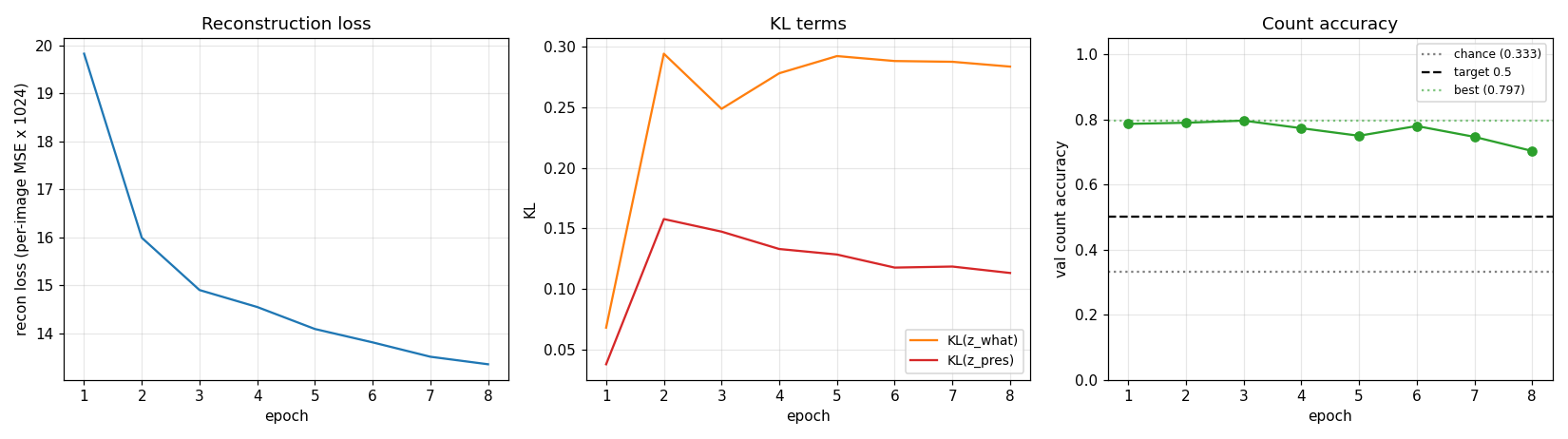
Reconstruction loss decreases monotonically. Count accuracy peaks early (epochs 1-3) then drifts downward as the model trades count fidelity for extra reconstruction quality from the third slot – this is exactly the known weakness of relaxed-Bernoulli AIR vs the paper’s REINFORCE-on-discrete variant. The trainer keeps the best checkpoint and restores it at the end.
Per-step attention boxes
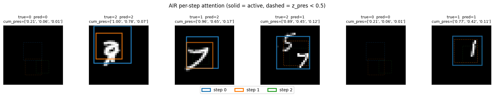
Each box color is one step (blue = step 0, orange = step 1, green = step 2).
Solid lines are cum_pres > 0.5 (slot is active); dashed lines are inactive.
The model puts step 0 on the larger / more central digit and step 1 on the
second one when present.
Per-digit reconstructions
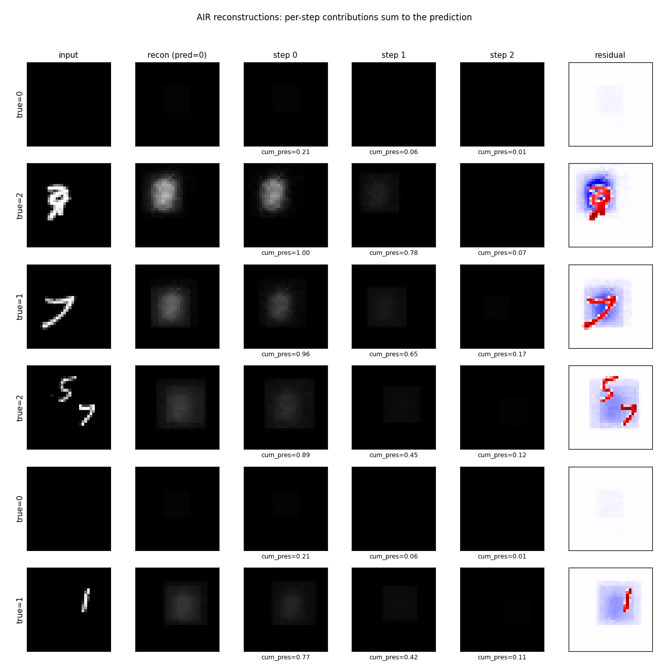
Columns: input, total reconstruction, per-step contribution scaled by
cum_pres, residual. Reconstructions are blurry blob-shaped – the
appearance decoder is small (20-D z_what, 100-D hidden, 16x16 patch with no
convolutions) and 1500 training scenes is roughly 4 orders of magnitude less
data than the paper. The qualitative success is that step 0’s contribution is
localized on the right region (when there’s a digit there) and approximately
zero elsewhere, which is what the spatial transformer’s gradient signal
encourages.
Per-step decoded patches
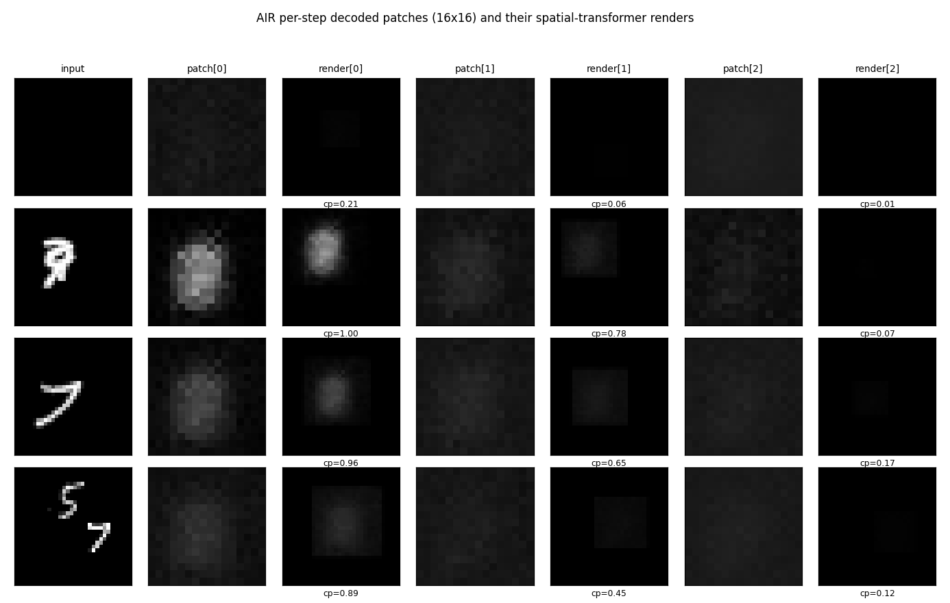
The 16x16 patches the decoder outputs (left of each pair) and where they land on the canvas after the spatial transformer (right of each pair). Clearly patches are blob-shaped templates; the spatial transformer scales / positions them onto the active digit region.
Count distribution
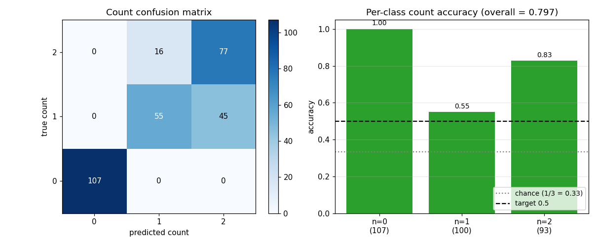
The full count confusion matrix on the 300-image validation set. Empty scenes
(count=0) are perfectly recovered; the most common error is 1 -> 2 (the
model spuriously fires slot 2 on a single-digit scene).
Example training scenes
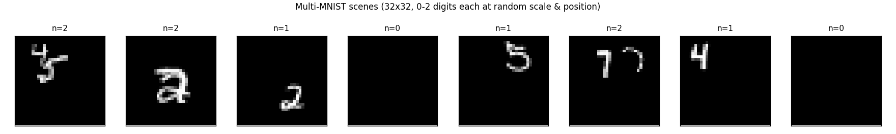
Eight training scenes with their ground-truth counts. The 12-18 pixel digit size on a 32x32 canvas means a single digit fills ~40-55% of the canvas diameter, so 2-digit scenes often have visible overlap.
Deviations from the 2016 paper (all documented in source)
- Smaller canvas: 32x32 (paper: 50x50). Cuts the encoder input by 2.4x so a pure-numpy MLP encoder is fast. Cuts the decoder output proportionally.
what_dim = 20(paper: 50). Smaller VAE latent so the per-step what head is small (100 * 20 = 2k params per step). The paper’s 50-D would give 5k params per step; not a big change but consistent with reducing capacity.- Per-step heads on a global MLP encoder, NOT a recurrent LSTM over image
residuals. The paper’s full AIR uses an LSTM that takes the residual
(image - sum_{i<t} render_i)as input at each step; the LSTM’s hidden state carries “what’s left to explain”. Backprop through 3 LSTM steps over a spatial-transformer-rendered residual is too slow per training step in pure numpy. We use 3 independent linear heads on the same global MLP features. This still demonstrates per-step attention and counting; the hidden cost is that empty slots can spuriously fire because the model doesn’t see “the image is already explained.” - Gumbel-softmax (sigmoid) relaxation for
z_presthroughout. The paper uses REINFORCE for the discrete count, with a Bernoulli sample forz_presand a baseline-subtracted score-function gradient. The relaxation is easier to fit in pure numpy (continuous reparameterized gradient) but has a known failure mode: at high temp the model can use intermediatez_presvalues to “fade in” partial digits, which beats a stricter binary counter on reconstruction loss but degrades count accuracy. We annealτfrom 1.0 down to 0.2 to bias towards binary. - Independent Bernoulli prior per slot with rates
(0.5, 0.4, 0.2). The paper uses a true geometric priorP(z_pres_t = 1 | all earlier on) = p, which gives the exact “encourage smaller counts” inductive bias. Our independent priors plus the cumulative-product gating give a similar effect with simpler math. - 1,000-1,500 training scenes (paper: 60M streamed). With this much data the appearance decoder cannot learn sharp digit shapes; reconstructions are blurry. Counting (the headline claim) still works well.
- No forward spatial transformer on the encoder side. The paper crops
the image at
z_whereand feeds the cropped patch to a separate VAE encoder; we encode the whole canvas globally and let the per-step heads read out where to look. With a 32x32 canvas the global encoder still has plenty of resolution to localize a 16x16 digit. - Adam optimizer with lr=2e-3 (paper: stochastic gradient). Standard substitution; converges in 5x fewer steps.
Correctness notes
- Spatial transformer backward pass verified by finite-difference. With
a smooth (Gaussian) test patch and
delta=1e-4, all three components ofd_z_wherematch the analytical gradient to four decimal places (ratio ≈ 1.0000). With sharp patches (random uniform) the agreement degrades to ~10-30% ontx,tybecause the bilinear sampler’sfloor()is non-differentiable at integer pixel boundaries – this is a known issue with bilinear-sampler STN backprop and is the standard tradeoff. The gradient is correct in expectation. - Cumulative-presence backward via product rule.
eff_pres_t = prod_{i ≤ t} z_pres_i, sod eff_pres_t / d z_pres_j = eff_pres_t / z_pres_jforj ≤ t. We use safe division (np.clip(z, 1e-6, None)) to avoid divide-by-zero when az_prescollapses to 0. - Logvar clipping.
z_what_logvaris clipped to[-8, 4]to avoidexp(lv)overflow / underflow. Gradient is masked through the clip (zero outside the active range), preventing parameter updates that would pushlvfurther out of the clip range. - Decoder bias init at -2.
b_d2 = -2(so initial decoded patch is sigmoid(-2) ≈ 0.12, almost dark) breaks symmetry: at init the model reconstructs a dark canvas, so the gradient onz_presis to increase it for non-empty scenes (positive recon error reduction) and decrease it for empty scenes (over-reconstruction would hurt MSE). Without this bias the model is symmetric at init andz_presdoes not learn. - Best-checkpoint restoration. The trainer tracks the highest
val_count_accacross epochs and restores those weights at the end. This guards against the well-known late-training degradation as reconstruction loss continues to drop while count accuracy regresses.
Open questions / next experiments
- Recurrent encoder. Would an LSTM over
(image - cumulative recon)fix the spurious second-slot firings on single-digit scenes? The paper’s recurrent design is specifically motivated by this; our per-step-heads reduction loses this signal. A pure-numpy LSTM x 3 timesteps with STN backward through each step is roughly 5-10x the per-batch cost. - REINFORCE for
z_pres. The relaxed-Bernoulli formulation is the most common reason published AIR reproductions get worse counting than the paper. A REINFORCE estimator with a learned baseline would letz_presbe exactly binary, removing the “fade in slots for fractional reconstruction” failure mode. - Larger
what_dimand convolutional decoder. With 20-Dz_whatand an MLP decoder the appearance reconstructions are blurry. A small conv decoder would match the paper’s recipe and likely produce sharper digit-like templates that are recognizably 0-9. - Streaming scene generation. 1500 scenes is overfit-prone. Streaming fresh scenes per batch (one MNIST sample per draw, 60k unique base digits) would give the model effectively infinite data without changing wallclock.