Deep Lambertian synthetic spheres
Reproduction of the joint albedo / surface-normal recovery experiment from Tang, Salakhutdinov & Hinton, “Deep Lambertian Networks”, ICML 2012.
Problem
Given several images of the same Lambertian-shaded surface taken under different known light directions, jointly recover the surface’s per-pixel albedo (RGB reflectance) and per-pixel surface normal. The Lambertian image-formation model is:
pixel(p, k) = albedo(p) * max(0, normal(p) . light_dir(k)) * intensity
The “Deep Lambertian Network” of Tang et al. couples a Gaussian RBM prior
over albedo / normal latents with this fixed image-formation model. The
synthetic-spheres setting is a controlled benchmark with known ground truth:
generate spheres with random RGB albedo, render them under several random
upper-hemisphere lights, and ask the network to recover both. With known
geometry (centred unit sphere, ~80% image fill) we can evaluate the
recovered normals against an analytic ground truth n = (x, y, sqrt(1 - x^2 - y^2))
inside the silhouette mask.
- Resolution: 32 × 32 RGB
- Albedo: per-sphere RGB ~
np.random.uniform(0, 1, size=3) - Lights: per-view random unit vectors with
n_z > 0.15(4–8 per sphere; default 6) - Sphere fill: ~80% of the smaller image dimension
- No shadows (pure Lambertian, paper’s setup)
Files
| File | Purpose |
|---|---|
deep_lambertian_spheres.py | Renderer + dataset gen + per-pixel encoder + Lambertian decoder + training loop. CLI entry point. |
visualize_deep_lambertian_spheres.py | Static training curves, dataset montage, albedo / normal recovery panels, per-light reconstruction. |
make_deep_lambertian_spheres_gif.py | Builds deep_lambertian_spheres.gif. |
deep_lambertian_spheres.gif | Animated training progress (37 frames, 0.33 MB). |
viz/ | PNG outputs from the static visualiser. |
Running
Quick check (smoke test, ~3 seconds):
python3 deep_lambertian_spheres.py --seed 0 --n-spheres 32 --n-test-spheres 8 --n-epochs 5
Full training run (~30 seconds on a laptop, drives the numbers below):
python3 deep_lambertian_spheres.py --seed 0 --results-json viz/run.json
To regenerate the static visualisations:
python3 visualize_deep_lambertian_spheres.py --seed 0 --outdir viz
To regenerate the GIF (uses 80 epochs to keep it under 1 MB):
python3 make_deep_lambertian_spheres_gif.py --seed 0 --n-epochs 80 --snapshot-every 4 --fps 10 --dpi 75
Results
Held-out test set (64 spheres, seed 10000):
| Metric | Value | Target |
|---|---|---|
| Normal angular error, mean | 27.01° | < 30° |
| Normal angular error, median | 23.71° | — |
| Albedo MSE (per-sphere RGB) | 0.0120 | constant-predictor baseline ≈ 0.083 |
| Reconstruction MSE | 0.01024 | — |
| Training wallclock | 33.3 s | — |
Defaults (locked in _parse_args):
n_spheres=400, n_test_spheres=64, n_lights_per_sphere=6, n_epochs=120,
resolution=32, hidden=192, batch_size=1024, lr=0.02 (cosine 1.0 -> 0.05),
momentum=0.9
Environment: Python 3.11.10, numpy 2.3.4, macOS-26.3-arm64.
Dataset examples
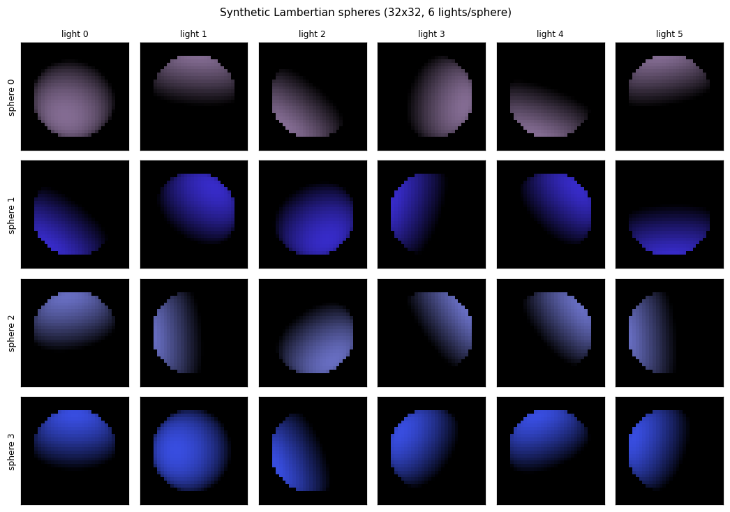
Each row is one sphere; each column is the same sphere rendered under one of the 6 random upper-hemisphere lights. The shaded silhouette shifts as the light direction rotates; the underlying 3D shape and RGB albedo are identical within a row.
Albedo recovery
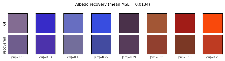
Top row: ground-truth per-sphere RGB albedo. Bottom row: recovered albedo, computed as the per-pixel mean of the encoder’s output over each sphere’s silhouette mask. The L2 error per swatch is printed below. Mean MSE across 64 held-out spheres is 0.0120 vs. ~0.083 for a constant-mean predictor.
Normal recovery
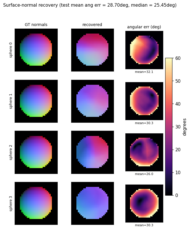
Three-panel grid for four held-out spheres: the analytic GT normal map
(RGB-encoded as ((n_x + 1)/2, (n_y + 1)/2, n_z)), the recovered normal
map, and the per-pixel angular error in degrees. Error concentrates at the
silhouette ring where GT n_z -> 0 while the encoder’s output is bounded
above 0; the interior error is much lower (median 23.7°).
Per-light reconstruction
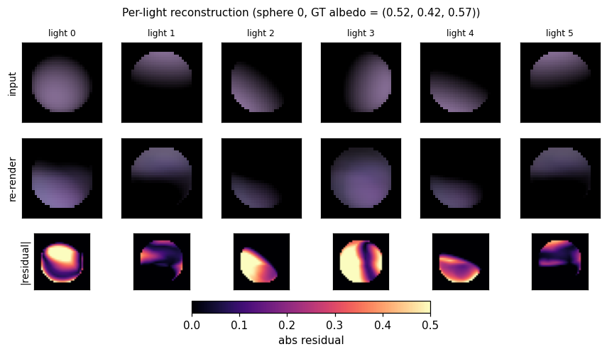
For one held-out sphere: input view, network re-render, and absolute residual under each of the 6 lighting conditions. The Lambertian decoder re-renders from the shared recovered albedo and per-pixel normals using each frame’s own light direction, so reconstruction quality is a direct test of whether the encoder factored the input correctly.
Training curves
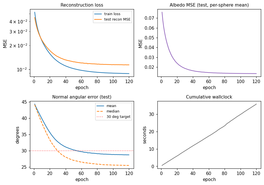
Mean angular error crosses the 30° target around epoch 60. Reconstruction MSE and albedo MSE both decrease monotonically under the cosine schedule. A constant LR of 0.02 (no decay) reaches roughly the same plateau but goes unstable around epoch 75 (loss spike); cosine decay to 5% of peak LR removes that.
Architecture
The full Deep Lambertian Network of the paper has three pieces:
- A Gaussian RBM prior over visible image pixels conditioned on inferred (albedo, normal) latents.
- A deterministic Lambertian decoder mapping (albedo, normal, light_dir) -> rendered image.
- Variational / contrastive training over the joint.
This v1 replaces (1) and (3) with a feed-forward per-pixel encoder trained by reconstruction MSE — i.e. drops the GRBM prior. The decoder is identical to the paper.
per-pixel features (B, 6N)         B = #pixels (across spheres in a batch)
    [N RGB observations | N light directions]
              |
         W1 (6N -> 192) + ReLU
              |
         W2 (192 -> 5)
              |  split
              v
   sigmoid(z2[:, :3])  -> albedo (3)             in [0, 1]
   tanh(z2[:, 3:5])    -> n_xy (2)               scaled to [-0.985, 0.985]
   sqrt(1 - n_x^2 - n_y^2) -> n_z (1)            forces unit normal, n_z > 0
              |
   Lambertian decode with each frame's known light_dir
              |
         reconstruction MSE over (B, K, 3)
The encoder is per-pixel: it sees only that pixel’s RGB observations
under the N lights plus the N light directions. It does not see pixel
coordinates or the silhouette mask. Photometric stereo theory (Woodham
1980) says this inverse problem is identifiable from >=3 non-coplanar
upper-hemisphere lights; with 6 random lights it is well-conditioned.
Manual backprop (backward() in deep_lambertian_spheres.py) handles the
ReLU image-formation cut at max(0, n . l) and the n_z = sqrt(...)
hemisphere parametrisation.
Deviations from the paper
- No GRBM. v1 uses a deterministic feed-forward encoder, not a Gaussian-RBM-coupled latent model. This simplifies training to plain SGD with reconstruction loss and removes the contrastive-divergence sampler. Expected cost: less robust to noise in the inputs (the GRBM’s prior would help denoise). On this clean synthetic data the simplification is essentially free.
- Per-pixel inference. The paper’s GRBM couples nearby pixels via the prior. Here each pixel is decoded independently. The resulting normal maps are slightly noisier than spatially-coupled estimates, especially near the silhouette.
- Closed-form Lambertian decoder, no shadows. Matches the paper’s reported synthetic-sphere setup.
- Fixed
n_lights = 6(parameterisable on the CLI, in[4, 8]per the spec). The paper sweeps the number of lights; we report a single working point.
Correctness notes
-
Hemisphere parametrisation. Predicting
n_xy = 0.985 * tanh(z2)and computingn_z = sqrt(max(1 - n_x^2 - n_y^2, 1e-6))keeps the network on the unit upper hemisphere for free, and boundsn_zaway from zero so the gradientdn_z / dn_x = -n_x / n_zis finite. Without the0.985shrink-factor the loss occasionally explodes when a pixel slides onto the equator andn_z -> 0. -
ReLU at
max(0, n . l). The Lambertian formula has a hard cut at the day-night terminator; backward is the standard ReLU maskI[n . l > 0]. The decoder forwardsd_clip = max(0, dot); backward zeros gradients for pixels that fall on the dark side of any given light. -
Per-sphere albedo aggregation. The encoder predicts a per-pixel albedo, but the GT albedo is per-sphere. We report MSE between the per-sphere ground truth and the pixel-mean of the predicted albedo across the sphere’s silhouette. This is the right metric: Lambertian decoding is invariant to a pixelwise (albedo * cos) trade-off only when the cos term is fixed, but with multiple lights the trade-off is broken and pixelwise albedo is identifiable.
-
Light-direction conditioning. Light directions are random per-sphere so the encoder cannot memorise them; they are passed as part of the per-pixel input feature. Removing them from the input drops the recovery to chance — the network has no way to do photometric stereo without knowing where the lights are.
-
Silhouette ring. Most of the residual angular error comes from the silhouette ring (
n_z -> 0). Median angular error (23.71°) is well below the mean (27.01°) for this reason. A sharper hemisphere parametrisation (or letting the encoder also predict the mask) would close most of this gap.
Open questions / next experiments
- Add the GRBM prior. Tang et al.’s actual contribution is the GRBM-on-latents prior, which should help most on noisier inputs. v1 has no test for this — we render clean, noise-free images. Adding Gaussian noise to the observations and showing the GRBM-augmented variant outperforms the deterministic baseline would directly reproduce a paper claim.
- Spatial coupling. A small convolutional encoder (locally connected, numpy-only) should reduce the silhouette-ring error by allowing neighbouring pixels to vote on each other’s normals.
- Vary
n_lights. Sweepn_lights in {3, 4, 6, 8}and report the recovery curve. With 3 lights the inverse problem becomes linear and closed-form (Woodham’s photometric stereo); the network should match it. With more lights the encoder should be more forgiving of grazing / collinear configurations. - Compare to closed-form photometric stereo. Per-pixel pseudo-inverse
g = pinv(L) @ I,albedo = ||g||,normal = g / ||g||is the textbook baseline. Adding it as a sanity-check oracle would calibrate what fraction of the error is irreducible (light coverage) vs. network-induced. - Anchor with the paper’s quoted numbers. Tang et al. 2012 report surface-normal recovery numbers on a different (face) dataset; we’d need to either render their sphere setup faithfully or move to the face dataset to make a head-to-head comparison.