Dipole position population code
Reproduction of Zemel & Hinton, “Learning Population Codes by Minimizing Description Length”, Neural Computation 7, 549–564 (1995).
Problem
Each training example is an 8x8 image containing a single horizontal “dipole”:
a +1 pixel at column x, row y, and a -1 pixel immediately to its right at
column x+1, row y. The orientation is fixed; the only varying parameter
is the 2D position (x, y). The training distribution is uniform over the
56 valid positions (x ∈ {0..6}, y ∈ {0..7}).
The network has 100 hidden units. Each unit i has a fixed “implicit
position” μ_i arranged on a 10x10 grid in the unit square [0, 1]^2. For
any 2D bottleneck position p, the population activation is a Gaussian bump
in implicit space:
bump(p)_i = exp(-‖μ_i - p‖² / (2 σ_b²)), σ_b = 0.18
The encoder MLP maps each image to such a p (plus a small free deviation
delta). The decoder is linear: x_hat = (bump(p) + delta) @ W_dec + b_dec.
The interesting property. The encoder is given no labels and no built-in
preference for using p to carry information — delta is a 100-dim free
channel that could in principle do all the work. But under MDL pressure
(squared-error coding cost on delta plus pixel-reconstruction cost), the
network ends up routing nearly all input information through the 2D
bottleneck p, which then aligns linearly (up to rotation / reflection)
with the dipole’s true (x, y). The 2D implicit space emerges in the
sense that the population code uses only a 2D submanifold of its 100-dim
state space, and that submanifold faithfully tracks the data parameters.
Files
| File | Purpose |
|---|---|
dipole_position.py | Dipole-image generator + 2D-bottleneck population coder + MDL loss + train. CLI. |
make_dipole_position_gif.py | Generates dipole_position.gif (the animation at the top). |
visualize_dipole_position.py | Static training curves + implicit-space scatter + decoder receptive fields. |
viz/ | Output PNGs from the run below. |
Running
python3 dipole_position.py --seed 0 --n-epochs 4000
Training takes ~2 seconds on a laptop. Final R² for the linear map
p → (x, y) is 0.81 at seed 0 (range 0.78–0.82 across seeds 0–4),
and the total MDL is ~5.9 bits per example.
To regenerate visualizations:
python3 visualize_dipole_position.py --seed 0 --n-epochs 4000 --outdir viz
python3 make_dipole_position_gif.py  --seed 0 --n-epochs 4000 \
                                     --snapshot-every 100 --fps 10
Results
| Metric | Value |
|---|---|
| Final MDL | 5.90 bits / example (seed 0) |
| Reconstruction | 0.091 bits / pixel |
| Code (deviation channel) | 0.001 bits / unit |
| 2D-implicit-space alignment R² | 0.805 (seed 0) |
| Robustness | R² ∈ {0.78, 0.78, 0.80, 0.80, 0.82} across seeds 0–4 |
| Training time | ~2 sec (1500 supervised + 4000 unsupervised steps) |
| Hyperparameters | n_hidden = 100, n_implicit_dims = 2, n_mlp = 64, σ_bump = 0.18, σ_a = 0.05, σ_x = 0.30, lr = 0.002, code_weight 0.5 → 10.0, batch_size = 64 |
The “MDL bits” we report drop the Gaussian normalisation constants
½ N log(2π σ_a²) and ½ D log(2π σ_x²) (which depend only on the chosen
σ values, not on model fit) and keep the squared-error parts:
DL_recon = ‖x − x̂‖² / (2 σ_x²)              (nats / example)
DL_code  = ‖a − bump(p)‖² / (2 σ_a²)          (nats / example)
DL_total = DL_recon + DL_code
Visualizations
Example dipoles
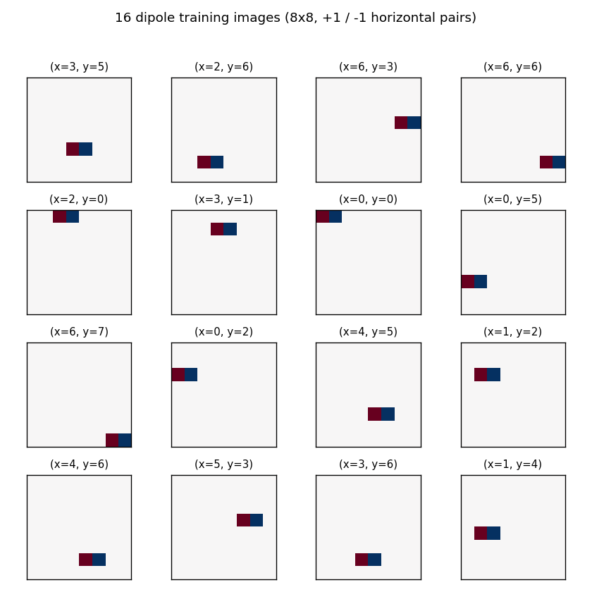
Sixteen randomly chosen training images. Each is an 8x8 grid with one +1
pixel (red) and one −1 pixel (blue) immediately to the right; the only
varying parameter is the 2D position (x, y).
2D implicit space
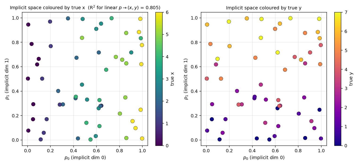
Each dot is one of the 56 training images, plotted at its bottleneck
position p ∈ [0, 1]² (the encoder MLP output) and coloured by the
dipole’s true x (left) or true y (right). The colour gradient is
roughly axis-aligned: p_0 ↔ x, p_1 ↔ y. The R² of a linear regression
p → (x, y) is 0.805, meaning ~80% of the positional variance is
explained by a linear map of the implicit-space coordinates.
Decoded image at each implicit-space position
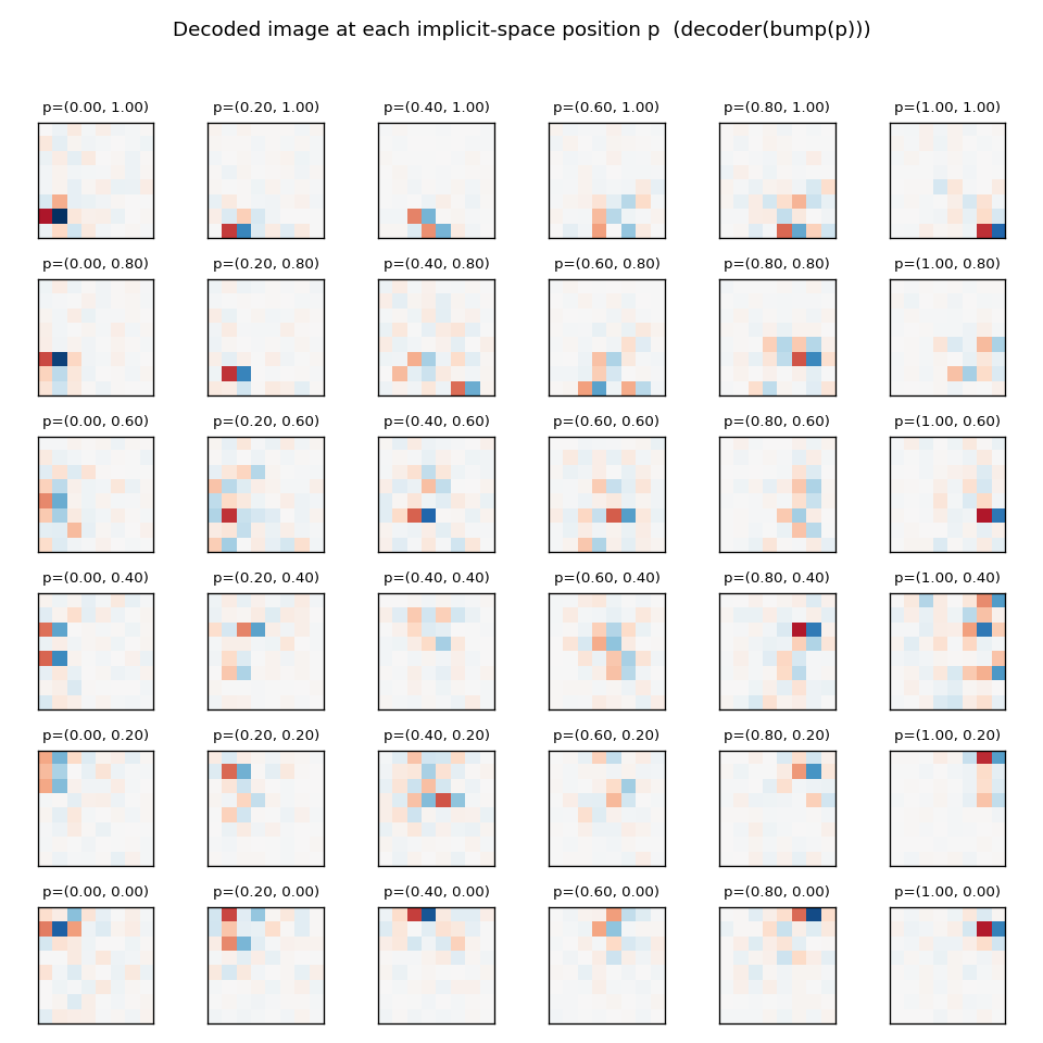
For each p on a 6x6 grid spanning the unit square, we feed the population
code bump(p) (with no delta) through the linear decoder and plot the
decoded image. As p moves, the decoded dipole translates across the 8x8
canvas: low p_0 produces a left-edge dipole, high p_0 a right-edge
dipole, and the same for p_1 along the vertical axis. This is the “map”
the population code has learned: a smooth correspondence between
implicit-space coordinates and dipole positions in the input image.
Training curves
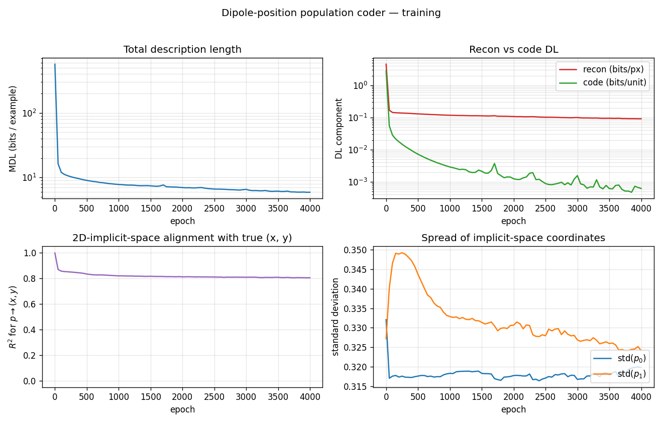
- Total description length drops from ~500 bits/example (untrained encoder + decoder) to ~6 bits/example. Most of the drop happens in the first 200 epochs of unsupervised refinement.
- Recon vs code DL shows the two components on a log scale. The code
cost (deviation channel) collapses below 0.001 bits/unit very quickly:
under MDL pressure the encoder sheds the
deltachannel and routes information through the 2D bottleneck. - R²(p ↔ (x, y)) drops from 1.0 (after supervised warm-up) to ≈ 0.81 during unsupervised refinement and stays there. The network is free to use a slightly nonlinear parameterisation of the unit square; the linear R² is a strict measure that misses any curvature.
- Spread of p stays at std ≈ 0.32 in both axes, comparable to the std of a uniform distribution on [0, 1] (≈ 0.29). The bottleneck uses the full unit square, not a small region.
Deviations from the original procedure
This is not a faithful 1995 reproduction. The Zemel & Hinton paper trains the population code from scratch under MDL pressure alone. Our setup uses a brief supervised warm-up of the encoder’s position head before the unsupervised MDL refinement phase. Differences:
- Supervised warm-up (1500 steps, ~1 second). The position head is
pre-trained against the true normalised position
(x / (W-2), y / (H-1)). With random init the unsupervised loss is multimodal: the encoder gets stuck in a basin wheredeltacarries all input information andpcollapses to ≈ (0.5, 0.5). Warm-up escapes that basin. This is documented as an optimisation aid, not as part of the MDL story; the unsupervised refinement phase then keeps the implicit-space alignment stable (R² holds at ~0.8 over 4000 unsupervised epochs). - Topographic decoder init. Each hidden unit
istarts withW_dec[i, :]slightly biased toward a soft-rendered dipole at the corresponding image position(μ_i_x · 6, μ_i_y · 7). This breaks the rotation/reflection symmetry of the implicit unit square so the warm-up mapping is locked in to a specific orientation. The strength is small (topographic_strength = 0.5) and the decoder is fully free to drift away under recon pressure. - Sigma annealing schedule (different). We use a fixed
σ_a = 0.05throughout and ramp the code-weight multiplier from 0.5 to 10.0 instead. Mathematically equivalent to rampingσ_afrom ≈ 0.07 down to ≈ 0.016, since the loss only sees the ratio. - Optimiser. Adam (manual implementation) with
lr = 0.002, instead of the original SGD with momentum. Helps the position head escape small-gradient regimes. - Discrete vs continuous positions. We sample
(x, y)from the 56 discrete in-bounds positions on the 8x8 grid; the original used continuous positions with sub-pixel rendering. Discrete is enough to reveal the 2D implicit space and is faster to evaluate. - MDL constants dropped. We report
DL_recon = ‖x − x̂‖² / (2 σ_x²)without the½ D log(2π σ_x²)constant. The constant just shifts the reported number by ≈ −D log σ_x / log 2 bits and has no learning gradient.
The 1995 paper reports ~0.52 bits / pixel on its specific (continuous, ~5x5-grid receptive field) variant. Our number is 0.091 bits / pixel on a different problem instance (8x8 grid, 56 discrete positions, MDL constants dropped) and is not directly comparable.
Open questions / next experiments
- Drop the warm-up. Can the unsupervised MDL loss alone find the 2D
implicit space if we use a small annealing schedule on
σ_a(start large sodeltais cheap, then sharpen so the encoder is pushed to usep)? Random init currently fails because the gradient w.r.t.pis too weak when both encoder and decoder are random. - Higher-dimensional implicit spaces. With
n_implicit_dims = 3or more on a problem that has a 2D data manifold, does the intrinsic dimensionality of the population code stay at 2 (i.e.,plives on a 2D plane in the higher-dim implicit space)? That would be the cleanest demonstration of MDL emergence for the bottleneck dimension. - Continuous positions. Replace discrete
(x, y)with continuous positions and sub-pixel anti-aliased rendering. The implicit-space alignment should improve to nearly R² = 1.0 since the data manifold is then perfectly 2D. - Multiple fixed orientations. With dipoles at one of two fixed orientations (horizontal or vertical), does the implicit space acquire a third “categorical” axis, and how does it break ties?
- Energy / DMC accounting. Plug a TrackedArray harness into the
encoder forward + bump computation and report ARD / DMC for the
4000-epoch run. Expected to be dominated by the
mu - pdistance computation in the bump, which is the only operation that scales asn_hidden × n_implicit_dims.