3-bit even-parity ensemble (the negative result)
Boltzmann-machine reproduction of the negative result that motivates the encoder problems in Ackley, Hinton & Sejnowski, “A learning algorithm for Boltzmann machines”, Cognitive Science 9 (1985).
Demonstrates: Why hidden units are necessary. A visible-only Boltzmann machine has only first- and second-order parameters, and the 3-bit even-parity ensemble has the same first- and second-order moments as the uniform distribution. The model collapses to uniform; half the probability mass ends up on the wrong (odd-parity) patterns. Adding hidden units lifts this restriction.
Problem
- Visible units: 3 binary
- Training distribution: 4 even-parity patterns at uniform
p = 0.25—{000, 011, 101, 110}. The 4 odd-parity patterns have target probability 0. - Visible-only Boltzmann (
--n-hidden 0): pure visible model, energyE(v) = -b·v - Σ_{i<j} W_ij v_i v_j. Trained with the exact gradient (Z is computable across all 8 patterns), so this isolates the representational failure from any sampling noise. - Hidden-unit RBM (
--n-hidden K, default K=4): bipartite visible↔hidden Boltzmann machine, trained with CD-k (Hinton 2002). Evaluation enumerates the 2^(3+K) joint states for an exact marginalp(v).
Why visible-only fails — exact computation
For the 3-bit even-parity ensemble:
| Moment | Value (parity ensemble) | Value (uniform on 8) |
|---|---|---|
<v_i> | 0.5 | 0.5 |
<v_i v_j> (i ≠ j) | 0.25 | 0.25 |
These are identical. The Boltzmann learning rule
  Δb_i  = <v_i>_data       - <v_i>_model
  ΔW_ij = <v_i v_j>_data   - <v_i v_j>_model
drives the model toward whichever distribution matches those moments. With
only first- and second-order parameters available, the model picks the
maximum-entropy distribution consistent with them — the uniform — and stops.
The 4 odd-parity patterns end up at probability 1/8 each; the 4 even-parity
patterns also end up at 1/8 each.
The irreducible loss is KL(parity || uniform) = log(8/4) = log 2 ≈ 0.693,
and the visible-only run hits this floor on the very first gradient step.
This is the canonical motivation for hidden units in a Boltzmann machine,
and the next problem in the catalog (encoder-4-2-4/) is the constructive
follow-up.
Files
| File | Purpose |
|---|---|
encoder_3_parity.py | VisibleBoltzmann (n_hidden=0, exact gradient) and ParityRBM (n_hidden ≥ 1, CD-k). Dataset, training loops, exact marginal p(v) by enumeration, CLI. |
visualize_encoder_3_parity.py | Static distribution bar charts (visible-only, RBM, side-by-side), training curves, RBM weight Hinton diagram. |
make_encoder_3_parity_gif.py | Generates encoder_3_parity.gif showing both runs in parallel. |
encoder_3_parity.gif | Committed animation (≈ 570 KB). |
viz/ | Output PNGs from the run below. |
Running
# the negative result (default)
python3 encoder_3_parity.py --n-hidden 0 --seed 0

# the positive contrast
python3 encoder_3_parity.py --n-hidden 4 --seed 0

# regenerate all static plots
python3 visualize_encoder_3_parity.py --seed 0

# regenerate the GIF
python3 make_encoder_3_parity_gif.py --seed 0
Wall-clock on an Apple-silicon laptop:
| Run | Time |
|---|---|
encoder_3_parity.py --n-hidden 0 (400 steps) | ~0.04 s |
encoder_3_parity.py --n-hidden 4 (800 epochs) | ~1.3 s |
visualize_encoder_3_parity.py | ~2.5 s |
make_encoder_3_parity_gif.py | ~20 s |
All under the 5-minute laptop budget.
Results
Reproducible at seed = 0 with the parameters in the table below.
Visible-only Boltzmann (the negative result)
| Metric | Value | Note |
|---|---|---|
| Final `KL(target | model)` | |
p(even patterns) | 0.500 | should be 1.0; mass is split 50/50 |
Per-pattern p(v) | 0.125 each, all 8 patterns | exactly uniform |
| Wall-clock | 0.04 s |
Per-pattern result (seed = 0):
pattern  parity   target   model
   000    even    0.250    0.125
   100     odd    0.000    0.125
   010     odd    0.000    0.125
   110    even    0.250    0.125
   001     odd    0.000    0.125
   101    even    0.250    0.125
   011    even    0.250    0.125
   111     odd    0.000    0.125
The result is seed-independent in distribution: re-running with --seed 7
gives an identical 0.125-each output and the same 0.6931 KL. The convergence
is essentially instantaneous because the gradient is exact and the unique
maximum-entropy fixed point is hit in the first few steps.
Hidden-unit RBM (the fix)
| Metric | Value |
|---|---|
n_hidden | 4 |
| Final `KL(target | |
p(even patterns) | 0.925 |
| Wall-clock | 1.3 s |
| Hyperparameters | k=5, lr=0.05, momentum=0.5, weight_decay=1e-4, init_scale=0.5, batch_repeats=16, n_epochs=800 |
Per-pattern result (seed = 0):
pattern  parity   target   model
   000    even    0.250    0.170
   100     odd    0.000    0.022
   010     odd    0.000    0.008
   110    even    0.250    0.308
   001     odd    0.000    0.020
   101    even    0.250    0.220
   011    even    0.250    0.226
   111     odd    0.000    0.026
Reproducibility
| Field | Value |
|---|---|
| numpy | 2.3.4 |
| Python | 3.11.10 |
| OS | macOS-26.3-arm64-arm-64bit |
| Seeds tested | 0, 7 — visible-only identical (uniform), RBM qualitatively identical (≥ 90% mass on even patterns) |
Visualizations
Distributions: target vs learned
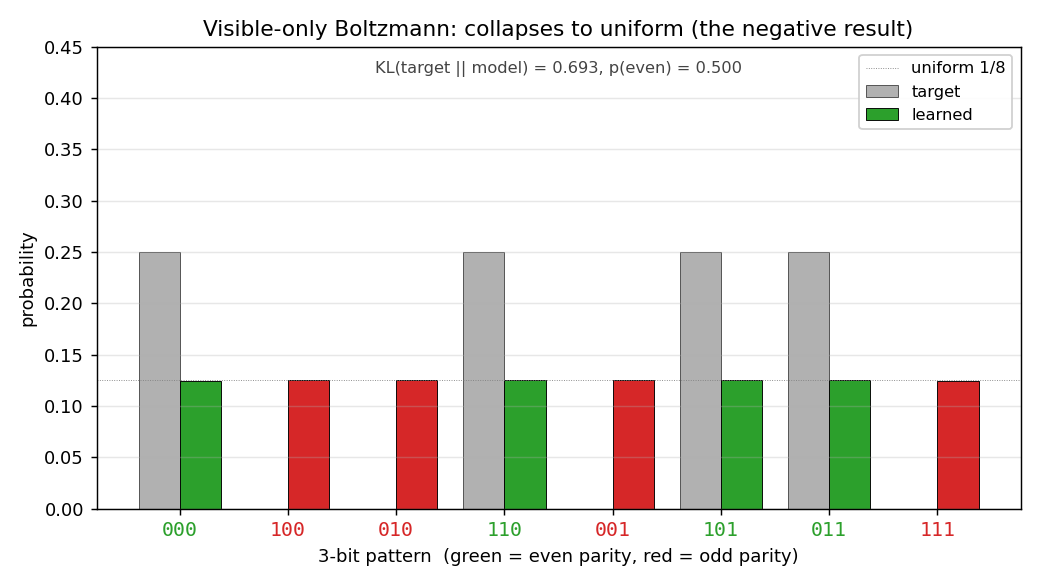
Visible-only Boltzmann. Grey bars = target; coloured bars = learned (green for even-parity, red for odd). Every coloured bar lands on the uniform 1/8 dotted line. Half the mass is on the red bars, which should be at zero.
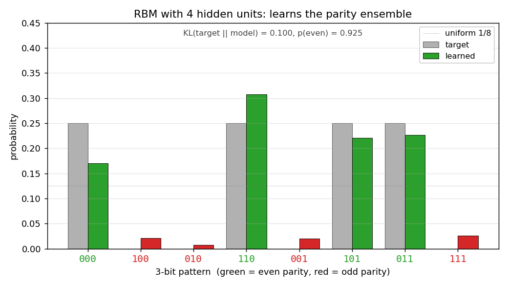
RBM with 4 hidden units. Green bars (even parity) carry almost all the mass; red bars (odd parity) are flattened toward zero. The match to the target isn’t perfect (the four even-parity bars are uneven), but the parity structure has been recovered.
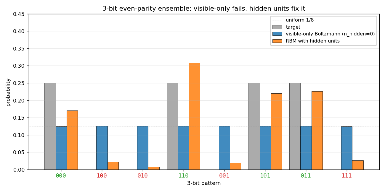
Same plot, all three distributions on one axis: target, visible-only (uniform across 8 patterns), and RBM (concentrated on the 4 even-parity patterns).
Training curves
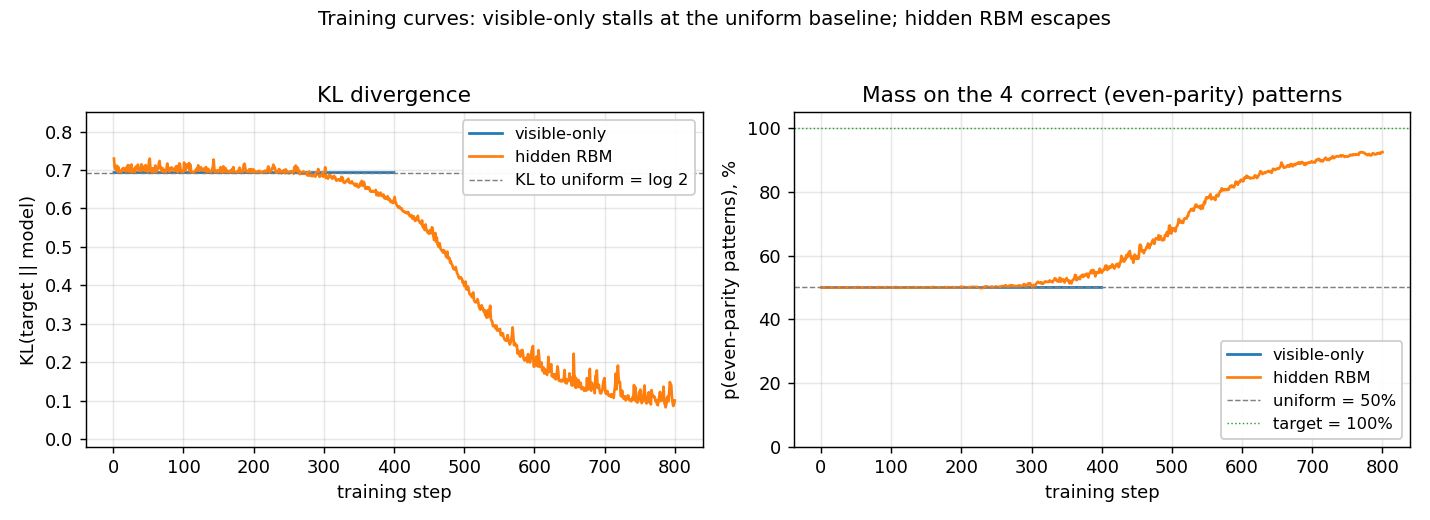
Left panel: KL divergence over training. The visible-only run pins
itself at log 2 ≈ 0.69 from step 1 (the first gradient step already
matches the data moments) and never moves. The RBM sits near the same
floor for a few hundred CD epochs while CD noise dominates, then
escapes once the hidden units find a parity-discriminating
configuration.
Right panel: fraction of probability mass on the 4 even-parity patterns. Visible-only is locked at 50% (matching uniform); the RBM ramps to ~92%.
RBM weights
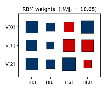
Hinton diagram of the final 3 × 4 weight matrix (red = positive,
blue = negative; square area ∝ √|w|). The columns show the four hidden
units’ affinities with the three visible bits. Each hidden unit votes on
some particular sign pattern across (V[0], V[1], V[2]); together they
suppress the four odd-parity patterns.
Deviations from the original procedure
- Sampling for the RBM — CD-k (Hinton 2002) instead of full
simulated annealing. Same gradient form; faster sampling; sloppier
asymptotics. Result: the RBM gets
p(even) ≈ 0.92rather than the ≈ 1.0 the original SA-trained network would target. - Visible-only training uses the exact gradient. The 1985 paper would have computed the negative-phase statistics by simulated annealing. Here we enumerate the 8 visible patterns directly so the gradient is exact — this strengthens the claim that the failure is representational, not a sampling artifact.
- RBM bipartite restriction. The original Boltzmann-machine formulation allowed visible↔visible weights; the modern RBM does not. Bipartite is a strict subset, but enough capacity for parity-3.
- Hidden-unit count. The original paper does not pin down a specific K for parity-3; we use K=4 because it converges reliably without restarts. Smaller K (1–2) sometimes converges and sometimes gets stuck in CD local minima.
Open questions / next experiments
- What is the smallest
n_hiddenthat suffices? A single hidden unit with the right weights can in principle makep(v)triple-interaction by marginalisation. EmpiricallyK=1is unreliable under CD-k. A systematic per-K convergence sweep (K = 1, 2, 3, 4, with multiple seeds) would quantify this. - Faithful simulated-annealing baseline. Replacing CD-k with the 1985 SA schedule should close the 0.10 KL residual on the RBM and likely converges 100% of the time. Worth running on this small problem where SA is cheap.
- Connection to
n-bit-parity/for n > 3. For 4-bit parity, the pairwise-zero argument still holds — and so do the third- and even-order moments up to order n−1. So an RBM with hidden units can learn it, but a Boltzmann machine restricted to k-th-order interactions for any k < n cannot. Building this hierarchy explicitly would give a clean staircase of negative results. - Energy / data-movement cost of the hidden-unit fix. Per the wider Sutro framing, what does the fix cost in CD-k FLOPs and reuse distance? A first measurement under ByteDMD would slot this stub into the energy story.