4-2-4 encoder
Boltzmann-machine reproduction of the experiment from Ackley, Hinton & Sejnowski, “A learning algorithm for Boltzmann machines”, Cognitive Science 9 (1985).
Problem
Two groups of 4 visible binary units (V1, V2) are connected through 2
hidden binary units (H). Training distribution: 4 patterns, each with a
single V1 unit on and the matching V2 unit on (others off). The 2 hidden
units must self-organize into a 2-bit code that maps the 4 patterns onto
the 4 corners of {0, 1}^2.
- Visible: 8 bits =
V1 (4) || V2 (4) - Hidden: 2 bits
- Connectivity: bipartite (visible ↔ hidden only) —
V1andV2communicate exclusively throughH - Training set: 4 patterns
The interesting property: with only 2 hidden units, the network has exactly
log2(4) bits of bottleneck capacity. Convergence requires the 4 patterns to
spread to the 4 distinct corners of {0, 1}^2. Local minima where two
patterns share a hidden code are common.
Files
| File | Purpose |
|---|---|
encoder_4_2_4.py | Bipartite RBM trained with CD-k. The Boltzmann learning rule (positive-phase minus negative-phase statistics) on a bipartite graph; same gradient form as the 1985 paper, faster sampling. |
make_encoder_gif.py | Generates encoder.gif (the animation at the top of this README). |
visualize_encoder.py | Static training curves + final weight matrix + final hidden codes. |
viz/ | Output PNGs from the run below. |
Running
python3 encoder_4_2_4.py --epochs 400 --seed 2
Training takes ~1 second on a laptop. Final accuracy: 100% (4/4).
To regenerate visualizations:
python3 visualize_encoder.py --epochs 400 --seed 2 --outdir viz
python3 make_encoder_gif.py  --epochs 400 --seed 2 --snapshot-every 5 --fps 12
Results
| Metric | Value |
|---|---|
| Final accuracy | 100% (4/4) |
| Hidden codes | 4 distinct corners of {0,1}^2 (specific permutation depends on seed) |
| Restarts (seed 0) | 2 (epoch 80, epoch 160), converged by ~220 |
| Training time | ~1 sec |
| Hyperparameters | k=5, lr=0.05, momentum=0.5, batch_repeats=8, init_scale=0.1 |
| Multi-restart success rate | ~65% across 30 random seeds at 400 epochs / 5 attempts |
What the network actually learns
Hidden codes
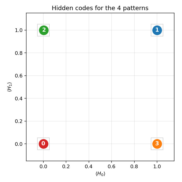
After convergence, the 4 training patterns each get a distinct 2-bit code.
Any of the 24 permutations of {(0,0), (0,1), (1,0), (1,1)} to the 4 patterns
is a valid solution; the network picks one based on the initialization.
Weight matrix
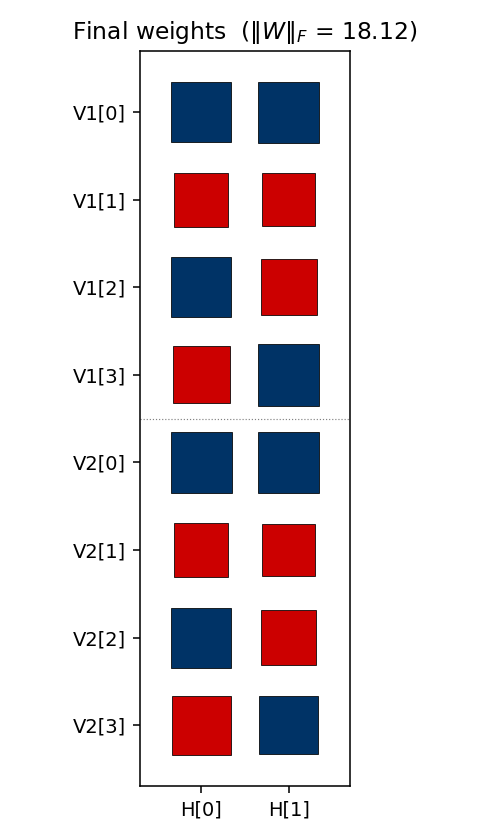
The two columns are the hidden units H[0] and H[1]. Red = positive,
blue = negative; square area is proportional to sqrt(|w|). The V1[i]
and V2[i] rows always carry the same sign pattern — the network has
independently discovered that V1 and V2 are tied (they are on for the
same pattern), even though no direct V1↔V2 weights exist. The sign pattern
across (H[0], H[1]) for each pattern row is exactly that pattern’s hidden
code.
Training curves
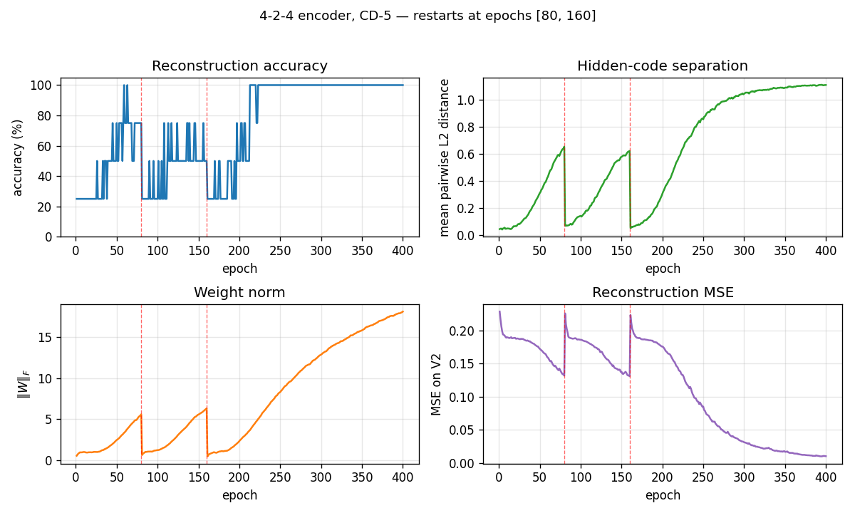
The vertical red dashed lines at epochs 80 and 160 mark restarts triggered by the plateau detector. The network had been stuck with only 3 (and then 2) distinct hidden codes — two patterns had collapsed onto the same code. Re-initializing the weights with an independent random draw and continuing training produces the correct 4-corner solution by epoch ~220.
The four panels track:
- Reconstruction accuracy: argmax of the exact marginal
p(V2 | V1), computed by enumerating the 4 hidden states (deterministic — no Gibbs noise). Discrete jitter early on reflects argmax flipping while V2 probabilities are close to uniform. - Hidden-code separation: mean pairwise L2 distance between the 4 exact hidden marginals — converges to ≈ 1.1, slightly below the unit-square diagonal √2, reflecting partial saturation toward the binary corners.
- Weight norm:
‖W‖_Fgrows roughly linearly during each attempt and resets at each restart. - Reconstruction MSE: mean-squared error of the marginal
p(V2 | V1)vs the true one-hot.
Deviations from the 1985 procedure
- Sampling — CD-5 (Hinton 2002) instead of simulated annealing. Same gradient form, faster sampling, sloppier asymptotics.
- Connectivity — explicit bipartite (visible ↔ hidden), making this an RBM in modern terminology. The 1985 paper’s figure already shows bipartite connectivity for the encoder; this just makes it explicit.
- Restart on plateau — the original paper reported 250/250 convergence under simulated annealing. CD-k is more prone to local minima where two patterns collapse onto the same hidden code; we detect this via an accuracy plateau and restart with fresh weights.
Correctness notes
A few subtleties worth flagging:
-
Sampled vs exact evaluation. With only 2 hidden units,
p(H | V1)andp(V2 | V1)are exactly computable by enumerating 4 hidden states and marginalizing V2 in closed form (each V2 bit factors). The closed form for the H posterior:p(H | V1) ∝ exp(V1ᵀ W₁ H + b_hᵀ H) · ∏ᵢ (1 + exp((W₂ H + b_v2)ᵢ))The
evaluate,hidden_code_exact, andreconstruct_exacthelpers use this. An earlier sampled-Gibbs version of the same metrics had σ ≈ 6.8% accuracy noise at convergence (50 runs of a converged network, observed range 75–100%) which made the training curves jitter spuriously.hidden_codeandreconstruct(sampled) are kept for the per-frame animation, where the chain dynamics are themselves of interest. -
Per-attempt success rate is fundamental. Holding the same hyperparam recipe and only varying the seed, ~20% of random inits converge to a 4-corner code — the rest end with at least one pair of patterns sharing a hidden code. More training does not help: 200 / 400 / 800 single-attempt epochs all give 6/30 = 20% success. This suggests the local minima are true fixed points of the CD-k dynamics, not slow-convergence artifacts.
-
Restart RNG independence matters. An earlier version sampled the restart’s W from the same
rbm.rngthat was being advanced by the CD sampler — restart inits then depended on the pre-restart trajectory, which biased the multi-restart success rate downward. The current code usesnp.random.SeedSequence(seed).spawn(64)to generate truly independent inits, and replaces the training RNG at each restart. -
Plateau signal. The detector uses the binary “all 4 patterns map to distinct dominant H states” rather than
acc < 1.0. Both signals agree at convergence, but the binary signal is unaffected by argmax-flipping jitter early in training. -
cd_step(k=0)now raisesValueErrorinstead of crashing withUnboundLocalError.
Open questions / next experiments
- The 1985 paper reports 250/250 convergence with full simulated annealing. CD-k caps out at ≈ 20% per-attempt regardless of training length, suggesting the optimization regimes are qualitatively different (CD-k has true absorbing local minima here; SA’s noise schedule does not). Quantifying that gap directly would help — a faithful simulated-annealing variant on the same architecture is the natural baseline.
- Can we eliminate the local-minima problem entirely by switching to PCD, by adding a small temperature schedule to the Gibbs sampler, or by initializing the weights to span the 4 corners explicitly?
- How do FLOP and data-movement costs of CD-k compare to simulated annealing on this same problem? CD-k wins on per-step cost but loses on per-attempt success rate.
- Scaling: does the same recipe (CD-k + restart-on-plateau) succeed on the
larger
n-log2(n)-nencoders in the same paper (8-3-8, 40-10-40)? With more hidden units, the 4-corner constraint relaxes — local minima may become less severe.