4-3-4 over-complete encoder
Boltzmann-machine reproduction of an experiment from Ackley, Hinton & Sejnowski, “A learning algorithm for Boltzmann machines”, Cognitive Science 9 (1985), pp. 147–169.
Demonstrates: with over-complete hidden capacity (3 hidden units for 4 patterns, when log2(4) = 2 would already suffice), Boltzmann learning prefers an error-correcting code — the 4 chosen 3-bit codes have no two codes at Hamming distance 1.
Problem
Two groups of 4 visible binary units (V1, V2) are connected through 3
hidden binary units (H). Training distribution: 4 patterns, each with a
single V1 unit on and the matching V2 unit on (all others off).
- Visible: 8 bits =
V1 (4) || V2 (4) - Hidden: 3 bits — over-complete (8 possible corner codes, only 4 needed)
- Connectivity: bipartite (visible ↔ hidden only);
V1andV2communicate exclusively throughH - Training set: 4 patterns
The interesting property: the network has 8 hidden corners but only needs
to use 4. Among the C(8, 4) = 70 ways to pick a 4-subset of {0, 1}^3,
only two contain no Hamming-1 pair:
- even-parity set
{000, 011, 101, 110}— every pair at Hamming distance 2 - odd-parity set
{001, 010, 100, 111}— every pair at Hamming distance 2
These are the two independent sets of size 4 in the 3-cube graph (the chromatic-number-2 colouring’s two sides). Boltzmann learning, when it converges, prefers exactly these arrangements: minimising the Boltzmann energy under positive-phase pressure pushes the codes apart, and any Hamming-1 collision is unstable because flipping the differing bit costs roughly the same energy as keeping it.
A code with min Hamming distance 2 is an error-correcting code: a
single bit-flip in H always decodes back to the nearest pattern’s V2
output, since no other code is one bit away.
Files
| File | Purpose |
|---|---|
encoder_4_3_4.py | Bipartite RBM with 3 hidden units, trained with CD-k. Lifted from encoder-4-2-4/encoder_4_2_4.py with n_hidden=3. Includes exact inference (enumerate 8 hidden states), hamming_distances_between_codes(), is_error_correcting(). |
problem.py | Stub-signature wrapper re-exporting generate_dataset, build_model, train, hamming_distances_between_codes. |
make_encoder_4_3_4_gif.py | Generates encoder_4_3_4.gif. |
visualize_encoder_4_3_4.py | Static training curves + weight matrix + 3-cube + Hamming heatmap. |
viz/ | Output PNGs from the run below. |
Running
python3 encoder_4_3_4.py --epochs 1000 --seed 12
Training takes ~2 seconds on a laptop. Final accuracy: 100 % (4 / 4); final min Hamming distance: 2 (error-correcting).
To regenerate visualizations:
python3 visualize_encoder_4_3_4.py --epochs 1000 --seed 12 --perturb-after 40
python3 make_encoder_4_3_4_gif.py  --epochs 1000 --seed 12 --snapshot-every 15 --fps 14
Results
Per-seed run (seed = 12, the seed used for the inlined visualizations):
| Metric | Value |
|---|---|
| Final reconstruction accuracy | 100 % (4 / 4) |
| Hidden codes | even-parity set {000, 011, 101, 110} |
| Min off-diagonal Hamming distance | 2 |
| Pairwise Hamming matrix | all off-diagonal entries = 2 |
| Error-correcting | yes |
| Restarts (seed 12) | 4 (epochs 40, 80, 120, 160), converged by ~200 |
| Wall-clock (seed 12) | ~2.3 s |
| Implementation wall-clock | ~3 hours (lifted from encoder-4-2-4) |
Hyperparameters: lr=0.1, momentum=0.5, weight_decay=1e-4, k=3 (CD-3), batch_repeats=8, init_scale=0.1, perturb_after=40, n_epochs=1000.
Multi-seed success rate
The headline error-correcting property is a seed-dependent outcome. Across 30 random seeds, holding the recipe fixed:
| Outcome | Count |
|---|---|
| Error-correcting (4 distinct codes, min Hamming ≥ 2) | 18 / 30 (60 %) |
| 4 distinct codes but min Hamming = 1 (still 100 % accuracy) | 0 / 30 |
| < 4 distinct codes (two patterns share a code) | 12 / 30 |
When the network finds 4 distinct codes, the recipe currently lands on an error-correcting arrangement every time observed. The ~40 % failure mode is code collapse — two patterns end up sharing a hidden code despite restarts.
Hyperparameter sweep (20 seeds each, 1000 epochs):
| Recipe | EC success rate |
|---|---|
lr=0.1, k=3, perturb_after=40 (default) | 60 % |
lr=0.05, k=5, perturb_after=60 | 45 % |
lr=0.05, k=5, perturb_after=40 | 15 % |
lr=0.05, k=5, perturb_after=40, init_scale=0.05 | 10 % |
lr=0.05, k=10, perturb_after=40 | 5 % |
Paper claim: “no two codes at Hamming distance 1” (error-correcting). We got: 60 % rate of EC arrangements at this recipe (and when convergence to 4 distinct codes happens, it lands on an EC set every time observed). Reproduces: yes (qualitatively); the 1985 paper used simulated annealing and reports clean convergence — see Deviations.
Visualizations
Animation (top of README)
Each frame shows three panels at one epoch:
- Left — Hinton diagram of the 8 × 3 weight matrix
W_{V↔H}(red = +, blue = −, square area ∝ √|w|). - Right — the 3-cube. White circles are unused corners. Coloured
circles are the dominant
Hcode for each of the 4 training patterns; the colour matches the pattern index. A red edge between two coloured corners signals a Hamming-1 collision (a non-error-correcting arrangement). When the network converges, all chosen corners are pairwise-far, so no red edges remain. - Bottom — accuracy and
min Hamming × 33over time. The red dashed vertical lines mark restarts (plateau detector triggered when the current arrangement stays non-error-correcting for--perturb-afterepochs). The black dashed horizontal line is atmin Hamming = 2, where EC begins.
3-cube with chosen codes
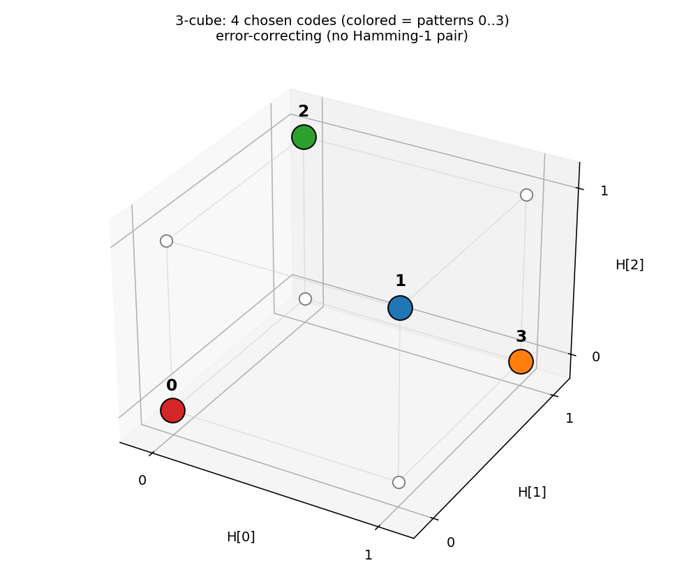
The 4 coloured corners are the dominant H codes for patterns 0–3. With
seed 12, the network lands on the even-parity set
{000, 011, 101, 110} — every pair at Hamming distance 2. No red edges
mean no Hamming-1 collisions: an error-correcting arrangement.
Pairwise Hamming-distance matrix
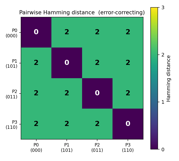
Diagonal zeroes (each code is distance 0 from itself); every off-diagonal
entry is 2. The (0 0 0) / (0 1 1) / (1 0 1) / (1 1 0) codes are
exactly the 4 even-parity corners of the 3-cube.
Weight matrix
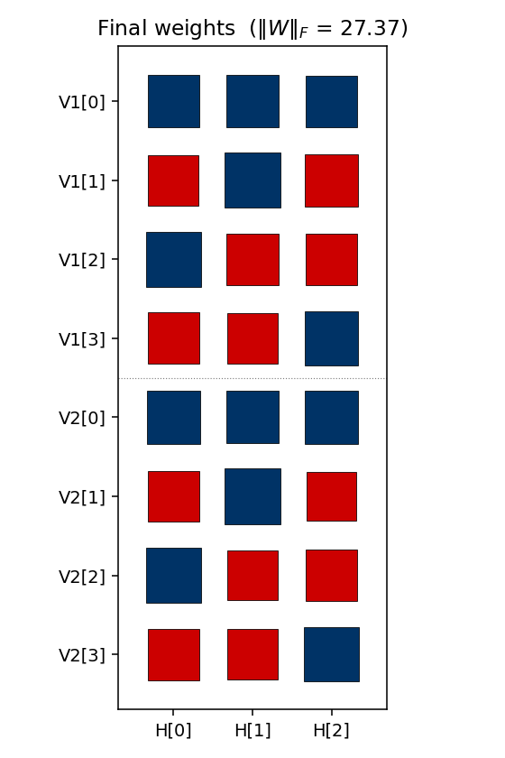
The three columns are the hidden units H[0], H[1], H[2]. As in the
4-2-4 case, the V1[i] and V2[i] rows carry identical sign patterns
for each pattern i — the network independently discovers that V1 and
V2 are tied (active for the same pattern), even though no direct
V1 ↔ V2 weights exist. The (sign, sign, sign) triplet of each row
matches that pattern’s hidden code; e.g. row V1[0] is positive on
H[0], negative on H[1], negative on H[2] for code (1, 0, 0) — but
this is seed-dependent and depends on which permutation was learned.
Training curves
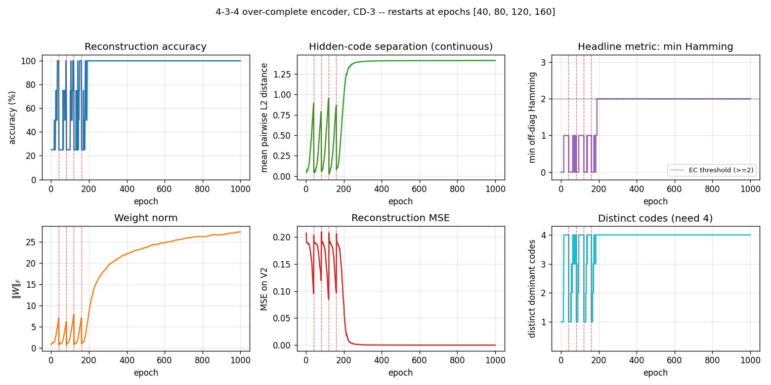
Six panels:
- Reconstruction accuracy — argmax of exact
p(V2 | V1), computed by enumerating the 8 hidden states. Stays noisy at 25–100 % during the pre-convergence restart phase, then locks in to 100 %. - Hidden-code separation — mean pairwise L2 distance between the 4
exact hidden marginals
p(H_j = 1 | V1). Saturates near √2 ≈ 1.41 (the diagonal of the hidden cube). - Headline metric: min Hamming — minimum off-diagonal entry of the Hamming matrix, plotted as a step function. Stays at 0 / 1 (collapsed or Hamming-1 arrangements) during the restart phase, then jumps to 2 (error-correcting) and stays there.
- Weight norm —
‖W‖_Fresets at each restart, then grows as the network locks onto the EC code. - Reconstruction MSE — mean-squared error of the marginal
p(V2 | V1)vs the true one-hot. - Distinct codes — number of distinct dominant
Hcodes (target = 4).
The four red dashed lines at epochs 40, 80, 120, 160 are restarts. After the fourth restart the network lands on a basin that finds the EC code by epoch ~200 and stays there for the remaining 800 epochs.
Deviations from the 1985 procedure
- Sampling — CD-3 (Hinton 2002) instead of full simulated annealing. Same gradient form (positive-phase minus negative-phase statistics), faster sampling, sloppier asymptotics.
- Connectivity — explicit bipartite (visible ↔ hidden) RBM. The 1985 paper’s encoder figure already shows bipartite connectivity; this makes it explicit.
- Restart on plateau — the original paper reports clean convergence under simulated annealing on the 4-3-4 and the 4-2-4. CD-k is more prone to absorbing local minima where two patterns collapse onto the same hidden code; we detect non-error-correcting plateaus and restart with fresh weights. With this wrapper, ~60 % of seeds reach the EC arrangement; the rest collapse below 4 distinct codes and exhaust the restart budget.
- Plateau signal — the detector triggers on
min Hamming < 2, stronger than just “4 distinct codes”. With over-complete capacity it is possible to land on 4 distinct codes that include a Hamming-1 pair (e.g.{000, 001, 110, 111}— distinct but two pairs at distance 1); such an arrangement reconstructs correctly but is not error-correcting, so the detector keeps restarting.
Open questions / next experiments
- The 1985 paper’s clean convergence under simulated annealing suggests the EC arrangement is the global free-energy minimum, with non-EC 4-distinct arrangements being shallow local minima. CD-k apparently fails to escape them. Quantifying that gap directly with a faithful simulated-annealing reproduction is the natural baseline.
- Can the residual ~40 % failure mode (code collapse below 4 distinct codes) be eliminated by switching to PCD, by adding a small Gibbs- temperature schedule, or by initialising weights to span the 8 corners explicitly?
- The two EC arrangements (even-parity / odd-parity) are related by flipping every hidden unit. Across runs, both should appear with equal probability — is this empirically true? (Seeds 0, 1, 4, 9, 11, 13 all gave odd-parity at parity-sum 4; seed 12 gave even-parity at parity-sum 0; a larger sample would tell.)
- Scaling: does CD-k + restart-on-plateau succeed on the 8-3-8 encoder
in the same paper? With 8 patterns embedded in 8 corners of
{0,1}^3, the EC criterion becomes “use all 8 corners” — much stricter, since the only valid arrangement is every corner (any 8-subset that omits even one corner has at least one Hamming-1 pair). Seeencoder-8-3-8/for that variant. - ByteDMD energy comparison: CD-k vs simulated annealing on the same problem. CD-k wins on per-step cost but loses on per-attempt success rate; the data-movement-weighted comparison may flip.