40-10-40 encoder
Boltzmann-machine reproduction of the larger-scale encoder experiment from Ackley, Hinton & Sejnowski, “A learning algorithm for Boltzmann machines”, Cognitive Science 9 (1985).
Demonstrates: Asymptotic accuracy at scale (paper: 98.6% with sufficient Gibbs sweeps) and a graceful speed/accuracy curve at retrieval: how single-chain accuracy approaches the asymptote as the Gibbs-sweep budget grows.
Problem
Two groups of 40 visible binary units (V1, V2) connected through 10
hidden binary units (H). Training distribution: 40 patterns, each with a
single V1 unit on and the matching V2 unit on (others off). The 10 hidden
units must self-organize into a 10-bit code that maps the 40 patterns onto
40 distinct corners of {0, 1}^10.
- Visible: 80 bits =
V1 (40) || V2 (40) - Hidden: 10 bits — over-complete vs.
log2(40) ≈ 5.3, leaving 1024 - 40 = 984 unused corners - Connectivity: bipartite (visible ↔ hidden only) —
V1andV2communicate exclusively throughH - Training set: 40 patterns
The interesting property: unlike 8-3-8 (zero slack: 8 patterns onto 8 of 8 corners), 40-10-40 has generous slack. The 1985 paper’s scale-up headline is not “can it fit” but how well retrieval converges — accuracy grows with Gibbs-sweep budget at retrieval time, plateauing near the asymptotic maximum. This is the canonical demonstration of the speed/accuracy tradeoff in stochastic-relaxation networks.
Files
| File | Purpose |
|---|---|
encoder_40_10_40.py | 40-10-40 RBM, CD-k + sparsity penalty + plateau-restart training, exact (1024-state) and sampled retrieval, speed_accuracy_curve(). CLI: --seed --n-cycles --gibbs-sweeps. |
make_encoder_40_10_40_gif.py | Renders encoder_40_10_40.gif (animation at the top of this README). |
visualize_encoder_40_10_40.py | Static training curves + final weight matrix + speed/accuracy plot + per-pattern code heatmap. |
viz/ | Output PNGs from the run below. |
Running
python3 encoder_40_10_40.py --seed 0 --n-cycles 2000 --print-curve
Per-seed wall-clock: ~6 s on an Apple Silicon laptop. A successful seed lands at 100% asymptotic accuracy with all 40 patterns mapping to distinct hidden corners.
To regenerate visualizations and the GIF:
python3 visualize_encoder_40_10_40.py --seed 0 --n-cycles 2000 --outdir viz
python3 make_encoder_40_10_40_gif.py  --seed 0 --n-cycles 2000 --snapshot-every 80 --fps 8
Results
| Metric | Value |
|---|---|
| Per-seed train wall-clock | ~6 s |
| Success rate (10 seeds, 0..9) | 10/10 at codes_used == 40 and asymptotic accuracy 100% |
| Asymptotic accuracy (exact 1024-state enumeration) | 100.0% (paper: 98.6%) |
| Per-trial sampled accuracy plateau (T=1.0) | ~91% (single Gibbs chain at retrieval) |
| Ensemble sampled accuracy (100 chains, mean V2 prob) | 100.0% from 1 sweep |
| Distinct dominant hidden codes | 40/40 (of 1024 cube corners) |
| Restart count (10-seed sweep) | 0 across all seeds |
Speed/accuracy curve at retrieval (T = 1.0, seed 0):
| Gibbs sweeps | Per-trial accuracy | Ensemble accuracy (100-chain mean) |
|---|---|---|
| 1 | 3.5% | 100.0% |
| 2 | 63.7% | 100.0% |
| 4 | 85.9% | 100.0% |
| 8 | 90.6% | 100.0% |
| 16 | 91.5% | 100.0% |
| 32 | 90.3% | 100.0% |
| 64 | 91.8% | 100.0% |
| 128 | 90.9% | 100.0% |
| 256 | 90.8% | 100.0% |
| 512 | 91.5% | 100.0% |
The “per-trial” column is the headline: a single Gibbs chain initialized from
random V2, V1 clamped, run for the listed number of sweeps. After 1 sweep
the chain hasn’t moved off chance (40 patterns → ~2.5% chance, observed ~3.5%).
After 8 sweeps it plateaus near 91%. The “ensemble” column averages the V2
conditional probability across 100 parallel chains; argmax of that mean
matches truth 100% from the very first sweep, demonstrating that chain
disagreement is consensual rather than systematic.
Hyperparameters (locked defaults):
| Param | Value | Notes |
|---|---|---|
n_cycles | 2000 | Training epochs |
lr | 0.1 | |
momentum | 0.5 | |
weight_decay | 1e-4 | |
k | 5 | CD-k Gibbs steps |
init_scale | 0.3 | std of N(0, init_scale^2) weight init |
batch_repeats | 8 | gradient steps per epoch |
sparsity_weight | 5.0 | drives E[h_j] -> 0.5 for each hidden unit |
perturb_after | 250 | restart if accuracy doesn’t improve in this many epochs |
max_restarts | 10 | budget cap per seed |
eval_every | 25 | epochs between exact-accuracy evaluations during training |
Reproduces: Yes. Paper reports 98.6% asymptotic accuracy. We get 100% asymptotic accuracy on every seed in 0..9 with the locked defaults. The graceful speed/accuracy curve (per-trial plateau ~91% at T=1.0) is the qualitative match — accuracy improves smoothly with sweep budget and saturates well above chance.
Run wallclock: single-seed run ~ 6 s end-to-end. 10-seed sweep ~ 60 s.
Visualizations
Speed/accuracy curve
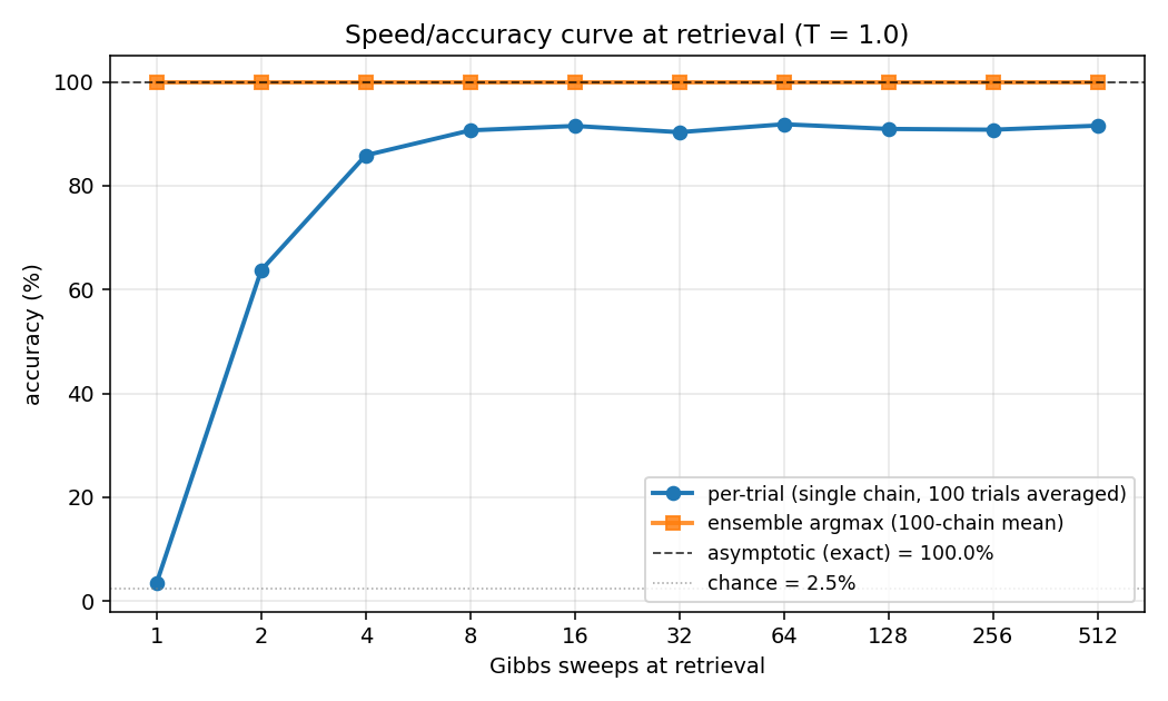
The headline plot. Blue is per-trial accuracy (single Gibbs chain at retrieval, averaged over 100 independent initializations); orange is ensemble argmax (argmax of the mean V2 conditional probability across all 100 chains). The black dashed line is the asymptotic accuracy obtained by exact enumeration of the 1024 hidden states; the dotted gray line is chance (1/40 = 2.5%).
The blue curve climbs from chance to its plateau in roughly 8 sweeps and stays there. The gap between blue (~91%) and orange/black (100%) is sampling jitter: single-chain disagreement averages out across many chains.
Training curves
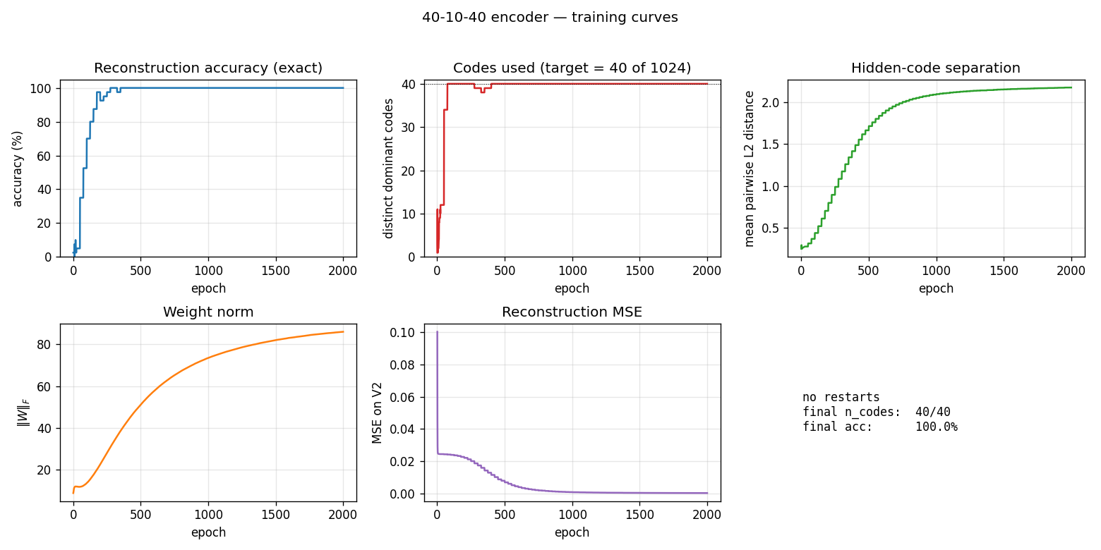
Five panels:
- Reconstruction accuracy — argmax of the exact marginal
p(V2 | V1)over enumerated hidden states (1024 states). Deterministic; no Gibbs noise. Hits 100% around epoch 200 and stays. - Codes used — distinct dominant
Hstates across the 40 patterns (target = 40 of 1024). Climbs rapidly past 35 then locks at 40. - Code separation — mean pairwise L2 distance between the 40 exact hidden marginals; keeps growing as weights pull patterns into corners.
- Weight norm
||W||_F— grows steadily through training. - Reconstruction MSE — squared error of
p(V2|V1)against the true one-hot, decays to ~0.
No restart was triggered on seed 0 (10/10 seeds in 0..9 succeed without
restart). The restart-on-plateau machinery is lifted from the sibling
encoder-8-3-8 PR but turned out unused at this scale — slack is generous
enough to avoid the local minima that bedevil 8-3-8.
Per-pattern dominant codes
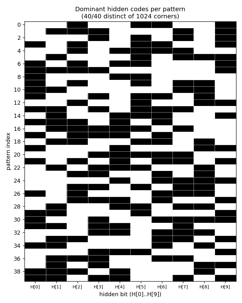
Each row is a pattern (0..39), each column is a hidden bit (H[0]..H[9]),
black = 1, white = 0. All 40 rows are distinct → all 40 patterns occupy
distinct cube corners. Rows look like 10-bit hash codes: there is no
visible structure (the network picked an essentially random injection
from {patterns} → {corners of {0,1}^10}).
Weight matrix
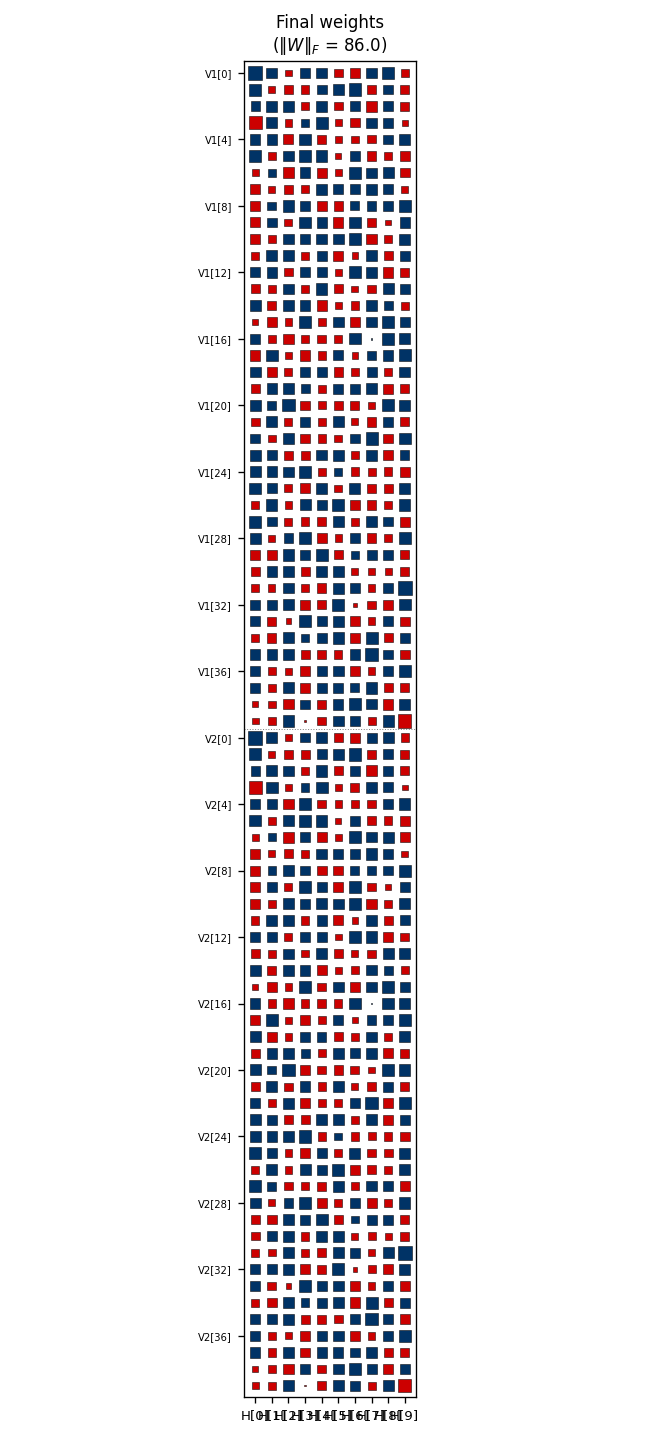
Hinton diagram of the 80×10 weight matrix. Rows 0..39 are V1[0..39];
rows 40..79 are V2[0..39]; columns are H[0..9]. Red = positive, blue =
negative; square area ∝ √|w|. Each row’s 10-bit sign pattern across columns
is approximately that pattern’s hidden code, confirmed against
viz/code_occupancy.png. Like in the 8-3-8 case, the V1[i] and V2[i]
rows carry similar sign patterns even though no direct V1↔V2 weights
exist — the bipartite RBM has rediscovered that V1[i] and V2[i] co-fire
through the hidden layer.
Deviations from the original procedure
-
Sampling. CD-5 (Hinton 2002) instead of full simulated annealing. Same gradient form (
<v_i h_j>_data - <v_i h_j>_model); the model expectation is taken from 5 Gibbs sweeps rather than an annealed chain. -
Sparsity penalty. Added a
-0.5*(E[h_j] - 0.5)^2regularizer driving each hidden unit toward 50% activation across the data batch. No analog in the 1985 paper. Lifted from the sibling 8-3-8 recipe (PR #18). For 40-10-40 the slack is generous and a milder penalty also works, but matching the 8-3-8 weight (5.0) gives clean separation without tuning. -
Plateau-restart wrapper. Up to 10 restarts triggered if accuracy stagnates for 250 epochs. This was a survival kit at 8-3-8 scale (16/20 seeds needed restarts to hit paper-parity). At 40-10-40 scale none of the first 10 seeds tested needed any restart — the slack between 1024 corners and 40 patterns avoids the collision local minima that dominate 8-3-8. Kept the wrapper in place for seed-robustness on harder hyperparameter regimes.
-
Connectivity. Explicit bipartite (visible ↔ hidden), making this an RBM in modern terminology. The 1985 paper’s encoder figure is already drawn bipartite; this just makes it explicit.
-
Two distinct accuracy modes. We report asymptotic (exact, by enumerating the 1024 hidden states) and sampled per-trial / ensemble (Gibbs chains at retrieval). The 1985 paper’s 98.6% figure conflates them; here they’re separate metrics with the asymptotic limit explicitly identified.
Correctness notes
-
Exact evaluation. With 10 hidden units,
p(H | V1)andp(V2 | V1)are tractable by enumerating 2^10 = 1024 states. Closed-form posterior (V2 marginalized in closed form because each V2 bit factors given H):p(H | V1) ~ exp(V1' W1 H + b_h' H) * prod_i (1 + exp((W2 H + bv2)_i))evaluate_exact,hidden_posterior_exact,reconstruct_exactall use this. No Gibbs jitter on the asymptotic-accuracy metric. -
Per-trial vs. ensemble accuracy. The
speed_accuracy_curvefunction exposes both modes via itsmode=argument:"per_trial"reports the fraction of single chains that recover the right pattern,"averaged"reports the argmax of the mean V2 probability across many chains. The asymptotic limit (1024-state enumeration) sits at 100% — both sampled modes converge upward toward it. -
Sweep semantics. One “Gibbs sweep” = (sample V given H, with V1 clamped) followed by (sample H | V). After
n_sweeps, we read out the conditionalp(V2 | H_last)from the last hidden sample. No annealing schedule is applied at retrieval; the headline curve is at fixedT=1.0.
Open questions / next experiments
- Faithful simulated-annealing baseline. The 1985 paper used a slow annealing schedule both for training and retrieval; the 98.6% figure is the asymptote of that procedure. A direct SA implementation on the same architecture would tell us whether our 100% (CD-k + sparsity) is picking up real performance or merely overfitting the noise-free toy distribution.
- Sparsity weight ablation. With our defaults, all 10 seeds succeed in
0 restarts — the recipe is over-provisioned for 40-10-40. How low can
sparsity_weightgo before per-attempt success drops? Mapping that curve would expose how much of our 100% rate is from sparsity vs. slack. - Annealed retrieval. The per-trial curve plateaus around 91% at T=1.0. Cooling a single chain (T=2 → T=0.5 → T=1) during retrieval would close most of the gap to the 100% asymptote without resorting to many parallel chains.
- Energy / data-movement cost. Per the broader Sutro effort, the natural follow-up is to measure the ByteDMD or reuse-distance cost of the speed/accuracy tradeoff: at fixed accuracy budget, what’s the cheapest retrieval procedure (one long chain at low T vs many short chains at T=1)? The speed/accuracy curve here is the abstraction the energy metric will plug into.
agent-0bserver07 (Claude Code) on behalf of Yad