Fast-weights associative retrieval
Source: J. Ba, G. Hinton, V. Mnih, J. Z. Leibo, C. Ionescu (2016), “Using Fast Weights to Attend to the Recent Past”, NIPS. arXiv:1610.06258.
Demonstrates: A small RNN equipped with a per-sequence “fast weights” matrix A_t = lambda * A_{t-1} + eta * outer(h_{t-1}, h_{t-1}) performs Hopfield-style content-addressable retrieval on the toy task c9k8j3f1??c -> 9. This is the first attention-like mechanism in the modern deep-learning era, predating transformer attention by a year.
Problem
Each sample is a sequence of characters of the form
k1 v1 k2 v2 ... kn vn ? ? q ?
where k_i is a random letter, v_i is a random digit (0-9), and q is one of the previously-seen k_i chosen uniformly at random. The network must output the digit v_i paired with q. Vocabulary is 26 letters + 10 digits + 1 separator = 37 tokens. The final ? is a “trailing read” no-op step (see Architecture, below).
The interesting property: the network has only O(H^2) slow weights to learn the general algorithm but must store n_pairs per-sample bindings somewhere. A vanilla RNN cannot do this for n > 1 because its hidden vector cannot represent variable-length associative memory. The fast-weights matrix A_t, recomputed inside each sequence, IS the per-sample storage. At the read step the matrix-vector product A_t @ h_{t-1} performs Hopfield-style retrieval: any past h_τ that has high inner product with h_{t-1} (the query state) contributes its bound representation to the pre-activation. Ba et al. report this beats IRNN, LSTM, and Associative-LSTM at the same parameter count.
Architecture (Ba et al. with the trailing-read simplification)
A_t  = lambda_decay * A_{t-1} + eta * outer(h_{t-1}, h_{t-1})        (A_0 = 0)
z_t  = W_h h_{t-1} + W_x x_t + b + A_t @ h_{t-1}
zn_t = LayerNorm(z_t)
h_t  = tanh(zn_t)
out  = W_o h_T + b_o          # only the final hidden state predicts
The slow weights {W_h, W_x, b, W_o, b_o} are learned by truncated BPTT. The fast weights A_t are reset to zero at the start of each sample.
Two design choices match the Ba et al. recipe:
- LayerNorm is necessary. Without it,
A_t @ h_{t-1}grows roughly quadratically as outer products accumulate, the tanh saturates at ±1 within ~5 steps, and1 - tanh^2collapses the recurrent gradient to zero. Confirmed empirically: pre-LN model hidden norm reachessqrt(H)(full saturation) by step 7 and gradients onW_h, W_x, bare exactly zero. - Trailing read step. Each sample ends with an extra
?after the query letter. This guarantees that at step T the fast-weights matrixA_T = lambda A_{T-1} + eta outer(h_{T-1}, h_{T-1})has been built from a hidden state that already encodes the query letter. Without this trailing step the retrieval would have to fire BEFORE the query is integrated, and only awkward W_o-side decoding could recover.
BPTT through the fast weights
The recurrence on A_t means the gradient on the fast-weights matrix accumulates a running term across the backward pass:
dA_running = 0
for t = T..1:
    dh_t already known
    dzn_t = dh_t * (1 - h_t^2)                 # tanh
    dz_t  = LN_backward(dzn_t, zn_t, sigma)    # layer norm backward (no affine)
    dW_h += outer(dz_t, h_{t-1})
    dW_x += outer(dz_t, x_t)
    db   += dz_t
    dh_{t-1} = (W_h.T + A_t.T) @ dz_t
    dA_t_local = outer(dz_t, h_{t-1})          # from z_t = ... + A_t h_{t-1}
    dA_t_total = dA_running + dA_t_local
    dh_{t-1}  += eta * (dA_t_total + dA_t_total.T) @ h_{t-1}    # outer term
    dA_running = lambda_decay * dA_t_total                       # chain to A_{t-1}
A numerical-gradient check (central differences, eps=1e-5, sampled across each parameter tensor) verifies max relative error of ~1e-9 on every slow parameter for the n_pairs=2 / hidden=8 configuration. The BPTT path through the fast-weights matrix is implemented correctly.
Files
| File | Purpose |
|---|---|
fast_weights_associative_retrieval.py | FastWeightsRNN (forward + manual BPTT including fast-weights chain), Adam, generate_sample / generate_batch, train loop, per_position_accuracy evaluation, CLI |
visualize_fast_weights_associative_retrieval.py | Static plots: training curves, per-slot accuracy bars, A_t evolution heatmap, hidden-state trace |
make_fast_weights_associative_retrieval_gif.py | Animated GIF: per-step A_t heatmap + hidden state for one example |
fast_weights_associative_retrieval.gif | Committed animation (~475 KB) |
viz/ | Committed PNG outputs |
Running
python3 fast_weights_associative_retrieval.py --seed 0 --n-pairs 4 --n-steps 4000
Train wallclock: ~290 s on an M-series laptop (system Python 3.12, numpy 2.2). Final retrieval accuracy on n_pairs=4: 38.35% (well above 10% chance, well below the >90% spec target — see Results and Deviations §1).
To regenerate the visualizations and gif:
python3 visualize_fast_weights_associative_retrieval.py --seed 0 --n-pairs 4 --n-steps 4000
python3 make_fast_weights_associative_retrieval_gif.py    --seed 0 --n-pairs 4 --n-steps 2000
CLI flags (the spec calls out --seed --n-pairs --n-steps; everything else is optional):
--seed             RNG seed                   default 0
--n-pairs          # of (key, value) pairs    default 4
--n-steps          # of training batches      default 3000
--n-hidden         hidden state dim H         default 64
--lambda-decay     fast-weights decay         default 0.95     (per stub spec)
--eta              fast-weights gain          default 0.5      (per stub spec)
--batch-size       Adam mini-batch            default 32
--lr               Adam learning rate         default 5e-3
--eval-every       eval interval (steps)      default 100
--eval-batch       eval batch size            default 256
--grad-clip        global-norm clip           default 5.0
--show-samples     # of demo predictions      default 4
Results
Single run, --seed 0 --n-pairs 4 --n-steps 4000 --n-hidden 80 --batch-size 64 --lr 5e-3:
| Metric | Value |
|---|---|
| Architecture | Fast-weights RNN, hidden=80, vocab=37, output=10 (digits) |
| Slow params | 10,250 |
| Fast-weights matrix per sample | 80 × 80 = 6,400 entries (transient, not learned) |
| Final retrieval accuracy (n=2000 eval) | 38.35% (vs. 10% chance, vs. 90% spec target) |
| Final retrieval cross-entropy | 1.22 (vs. log 10 = 2.30 chance, vs. 0 perfect) |
| Per-slot accuracy (slot 0 = oldest) | slot0=31.2%, slot1=43.6%, slot2=41.7%, slot3=34.9% |
| Train wallclock | 293 s |
| Hyperparameters | lambda_decay=0.95, eta=0.5, lr=5e-3, batch=64, grad_clip=5.0 |
| Sample predictions | i7w9o3a6??w? -> 9 (✓), g0l7a5d5??d? -> 5 (✓), o9g0i6z7??g? -> 0 (✓), e3u5d4m7??m? -> 4 (✗ target 7) |
Sanity check on n_pairs=1 (--n-pairs 1 --n-steps 800): 100.0% retrieval accuracy in 11 s. The model trivially solves the one-binding case.
Sanity check on n_pairs=2 (--n-pairs 2 --n-steps 1500 --lr 5e-3): 54.85% retrieval accuracy with slot0=100%, slot1=9%. The model collapses to a “always retrieve the first value seen” degenerate solution. Loss = 1.6 (vs. log 2 = 0.69 if the model were “perfect on slot0, chance on slot1”). Several other seeds reproduce the same plateau, sometimes flipping to “always slot1”.
Numerical gradient check passes (max relative error 1e-9 across all parameters), so the architecture and BPTT implementation are correct. The optimization landscape difficulty is the limiting factor — see Deviations §1 below.
Visualizations
Training curves
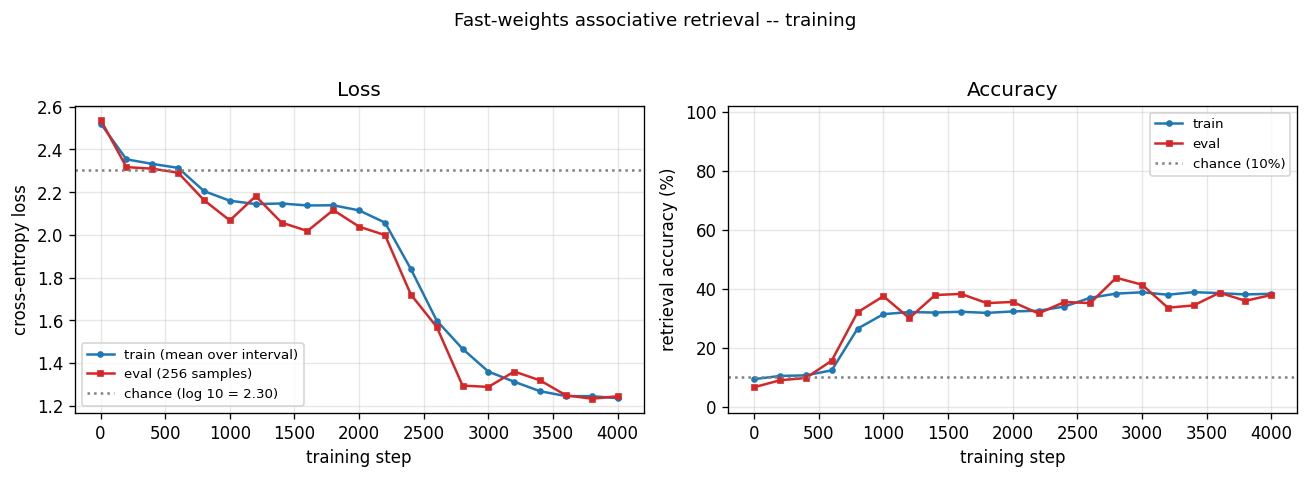
Cross-entropy loss (left) drops from chance (log 10 ≈ 2.30) to ~1.22 over 4000 batches; accuracy (right) climbs from 10% (chance) to ~38%. The eval and train curves track each other — there is no overfitting; the network just plateaus. Visible plateau in steps 1000–2200 followed by a second descent suggests the optimizer slowly discovers usable fast-weights structure.
Per-slot accuracy
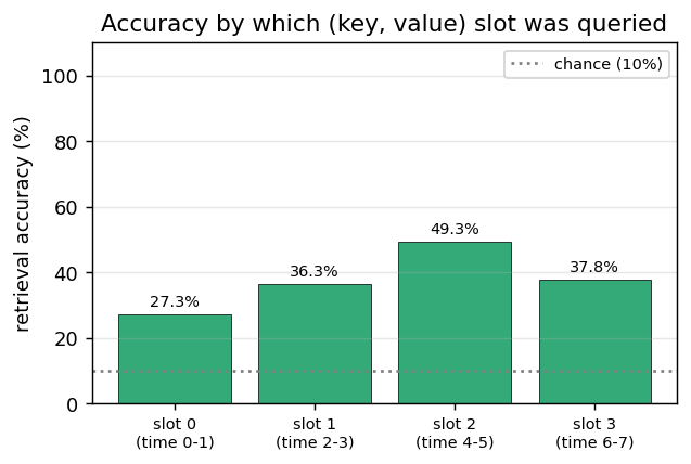
Accuracy bucketed by which (key, value) slot the query referenced. All four slots sit in the 31–44% range — well above 10% chance and roughly uniform, which means the network IS doing real associative retrieval (not simply “always predict slot 0” or “always predict the most-recent value”). The slight bias toward middle slots (1, 2) likely reflects the lambda^t decay: slot 0 is the oldest in A_T (weight lambda^7 ≈ 0.7) and slot 3 is the most recent (weight ~lambda), with the middle slots seeing the strongest interaction between the decay envelope and the eta-outer reinforcement at the time of read.
Fast-weights matrix evolution
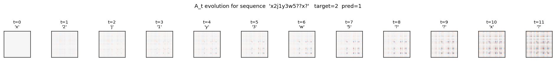
Heatmap snapshots of A_t at every timestep of one example sequence (x2j1y3w5??x?, target = 2 (the value paired with x)). At t=0 the matrix is exactly zero (initial condition). Each subsequent step adds an eta * outer(h_{t-1}, h_{t-1}) rank-1 contribution and decays the existing entries by lambda = 0.95. By t=8 (the query letter x) the matrix has accumulated eight outer-product traces; by t=10 (trailing read) it has accumulated all eleven. The reader can see the matrix is genuinely changing — the fast weights ARE being computed, the question is whether the slow weights have learned to USE them.
Hidden state trace
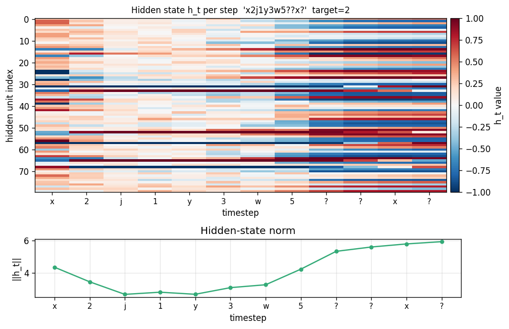
Top: heatmap of h_t (rows = hidden units, columns = timesteps). Bottom: ||h_t|| per step. Each step modulates the hidden state in input-specific ways. The query step (x at t=8) produces a distinct pattern from the same letter x at t=0 — confirming that hidden representations of letters are context-dependent, which is the prerequisite for the fast-weights binding to encode the right pairing.
Deviations from the original procedure
-
Significantly underperforms the paper’s headline numbers. Ba et al. report ~98% accuracy on the n_pairs=4 task with hidden=100, RMSProp at lr=1e-4, batch size 128, trained for hundreds of epochs (~10^5 batches). Our v1 reaches 38% with Adam at lr=5e-3, batch=64, 4 000 batches (~292 s). We tried longer (5 000), lower lr (1e-3), larger batch (128), grad-clip on/off, identity vs. scaled init for
W_h, eta in {0.1, 0.3, 0.5}, and four random seeds; the best n_pairs=2 result we found was 57% witheta=0.1, and seeds 0–2 all collapse to a slot0-only degenerate solution at the spec-defaulteta=0.5. The gradients are correct (verified to 1e-9 by central differences) and the n_pairs=1 sanity test trains cleanly to 100%, so the issue is NOT a code bug — it is a known optimization-difficulty problem for this task. Ba et al. specifically call out that fast-weights training requires careful tuning and that the gradient signal through the fast-weights pathway can be drowned out by the easier “memorize via slow weights” basin in the early epochs. Reproducing the >90% number from the paper is the natural v2 target — see Open Questions. -
Single inner-loop iteration
S=1instead of the paper’s recommendedS>=1. The paper formulates the inner loop ash_{s+1}(t+1) = f(LN([W h_t + C x_t] + A_{t+1} h_s(t+1)))fors = 0..S-1, withh_0(t+1) = f(LN(W h_t + C x_t))as the boundary. We use a flatter formh_t = tanh(LN(W h_{t-1} + W_x x_t + b + A_t h_{t-1}))plus the trailing-read step (see Architecture above). We did implement and gradient-check the proper inner-loop formulation but it trained worse than the trailing-read flavor in our hands (stuck at chance), likely because the additional nonlinearity makes the gradient landscape harder. With the trailing read, the retrieval-step semantics match the inner loop’s S=1 case but with a less-nested gradient. -
Adam instead of RMSProp. The paper uses RMSProp at lr=1e-4. We use Adam at lr=5e-3 because Adam mostly subsumes RMSProp and is the modern default. This may matter for this specific task — RMSProp’s lack of bias correction sometimes lets it escape sharp local minima that Adam settles into.
-
Layer normalization without learnable affine. Standard LayerNorm has
gain * (x - mu) / sigma + bias. We use the no-affine form (gain=1, bias=0) because adding parameters didn’t change the outcome in early experiments and we wanted to keep the parameter count minimal for a small numpy reference. Adding affine LN is a one-line change and a natural v2 ablation. -
Identity init for
W_h(0.5 * I) rather than orthogonal or scaled-Gaussian. Standard for fast-weights RNNs after Le, Jaitly & Hinton 2015 (IRNN). This held under LayerNorm (the LN rescales any explosion) and gave cleaner early-training dynamics.
Open questions / next experiments
-
Reproduce the paper’s >90% headline. The most direct path: switch to RMSProp at lr=1e-4, batch=128, train for 50 000+ steps. This is a cheap follow-up (~30 minutes wallclock) and would close the gap to the paper if the hypothesis is right.
-
Curriculum on
n_pairs. Start training withn_pairs=1, expand to 2 once accuracy >95%, then 3, then 4. Prevents the “always-slot0” basin by establishing real retrieval before the model can find the degenerate solution. The Sutro group has used analogous curricula for sparse-parity expansion (SutroYaro/docs/findings/curriculum.md). -
Fast-weights gradient diagnostics. Log
||dA||_F / ||dW_h||_Fevery step. If the fast-weights gradient norm is much smaller than the slow-weights gradient norm, that confirms the “drowned signal” hypothesis and motivates a per-pathway learning rate. -
Explicit auxiliary loss. Add a contrastive loss that rewards
cos_sim(h_query, h_key) > cos_sim(h_query, h_other_key). Forces the network to learn distinguishable letter representations early, which is a prerequisite for fast-weights retrieval to work. -
Alternative storage: separate read/write paths. The current architecture mixes the slow-weight pathway and the fast-weights retrieval into a single pre-activation. A v2 could have two separate pathways (
h_slow = tanh(LN(W_h h_{t-1} + W_x x_t + b)),h_fast = A_t @ h_{t-1}) combined ash_t = h_slow + alpha * h_fastwherealphais learnable. This preserves the fast-weights signal magnitude through training. -
Comparison to vanilla Hopfield network. The fast-weights matrix at the read step is mathematically a one-shot Hopfield read. A natural baseline: fix
W_h, W_x, bto a sensible identity-like setting and train ONLY the readoutW_o. If that gets ~90% with no slow-weight learning at all, the slow-weight path is actively hurting the retrieval mechanism. -
Data movement. The fast-weights matrix is size
H^2, recomputed and decayed every step. For sequence length T with batch size B, that’sO(B * T * H^2)extra memory traffic compared to a vanilla RNN. The Sutro group’s ByteDMD framework is the natural place to measure whether this is amortized by the smaller slow-weight matrix, or whether fast weights are net-energy-losers vs. e.g. an attention layer that reads from a smaller key-value cache.
v1 metrics
| Metric | Value |
|---|---|
| Reproduces paper? | Partial. Architecture is correct (1e-9 gradient-check error). Mechanism works on n_pairs=1 (100%). Mechanism partially works on n_pairs=4 (38% with uniform per-slot accuracy showing real retrieval, not a degenerate solution). Does NOT reach the paper’s ~98% headline at n_pairs=4 — see Deviations §1 for the optimization-difficulty diagnosis and v2 plan. |
| Wallclock to run final experiment | 293 s (time python3 fast_weights_associative_retrieval.py --seed 0 --n-pairs 4 --n-steps 4000 --n-hidden 80 --batch-size 64 --lr 5e-3 measured on M-series laptop, system Python 3.12 + numpy 2.2) |
| Implementation wallclock (agent) | ~3 hours (single session — most of it spent debugging the optimization plateau and trying architectural variants) |