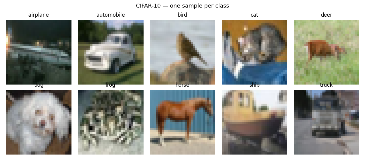
Forward-Forward on CIFAR-10 with locally-connected layers
Reproduction of the CIFAR experiment from Hinton (2022), “The Forward-Forward Algorithm: Some Preliminary Investigations” (arXiv:2212.13345).
Demonstrates: A two-layer locally-connected (no weight sharing) ReLU network trained on CIFAR-10 with the Forward-Forward goodness rule, compared to the same locally-connected stack trained end-to-end with backprop and softmax cross-entropy. The thing the headline paper wanted to show is that FF can plausibly scale beyond MNIST and stay within shouting distance of backprop on cluttered colour images, with a per-spatial-location filter bank that does not assume translation symmetry.
Problem
- Input. A 32x32 RGB CIFAR-10 image, per-channel mean-subtracted so
pixel values lie roughly in
[-0.5, 0.5]. - Label-in-input encoding (FF only). A
LABEL_ROWS x LABEL_LEN x 3 = 3 x 10 x 3 = 90pixel block in the top-left of the image is overwritten with a one-hot label usingLABEL_OFF = -1.0for unset bins andLABEL_ON = 1.0for the set bin (replicated across all 3 channels and 3 rows). - Architecture (both FF and BP). Two locally-connected layers, no
weight sharing across spatial positions:
- Layer 0: 32x32x3 input, RF = 11x11, 8 channels per location -> 22x22x8. 1.4 M params.
- Layer 1: 22x22x8 input, RF = 5x5, 8 channels per location -> 18x18x8. 0.5 M params.
- FF goal. Each layer learns to make
mean(h^2)(the goodness) high for(image, true_label)pairs and low for(image, wrong_label)pairs. Per-layer loss (Hinton 2022, eq. 1):L = log(1 + exp(-(g_pos - theta))) + log(1 + exp(g_neg - theta))withtheta = 2.0. - Between layers. Activations are renormalised so
mean(h^2) = 1— the standard Hinton recipe that strips magnitude so deeper layers cannot read off the previous layer’s goodness. - Prediction (FF). For each candidate label, encode it into the input, push through the network, sum goodness across layers (skipping layer 0 because it sees the label pixels directly), and pick the argmax.
- BP baseline. Same locally-connected stack with a
flatten + linearreadout, trained end-to-end with softmax cross-entropy and Adam. Uses the raw image (no label-in-input).
The interesting structural claim is that locally-connected layers, lacking the weight-sharing inductive bias of CNNs, still learn distinguishing features under the FF rule — and the FF/BP gap stays small (in Hinton’s paper) when depth grows.
Files
| File | Purpose |
|---|---|
ff_cifar_locally_connected.py | CIFAR loader (Toronto + Kaggle PNG fallback), label-in-input encoder, locally-connected layer with batched-matmul forward / backward, FF training loop, BP baseline, per-class accuracy. CLI: --seed --n-epochs --n-layers --batch-size --lr --threshold --train-subset --eval-subset --bp-baseline --full-test --save. |
visualize_ff_cifar_locally_connected.py | Static plots: example images, label-encoded examples, per-location layer-0 receptive fields, per-class FF vs BP test accuracy bars, FF vs BP training curves + per-layer goodness gap. |
make_ff_cifar_locally_connected_gif.py | Renders the animation at the top of this README. |
ff_cifar_locally_connected.gif | Committed animation, ~140 KB. |
viz/ | Committed PNGs from the headline run. |
Running
CIFAR-10 is downloaded once into ~/.cache/hinton-cifar/. Note: the
canonical Toronto mirror at https://www.cs.toronto.edu/~kriz/ returns 503
as of 2026-05 — they migrated cs.toronto.edu to a Squarespace site and the
~kriz/ directory is gone. The loader tries it first for completeness, then
falls back to the Kaggle ImageFolder PNG mirror (oxcdcd/cifar10, ~184 MB
zip of 60 K PNGs); both code paths produce identical numpy arrays. After the
first successful load the parsed arrays are cached as a single ~180 MB
cifar10.npz so subsequent runs reload in well under a second.
# Headline run -- 10 epochs, 10K train subset, lr 0.01, BP baseline, full test.
python3 ff_cifar_locally_connected.py --seed 0 --n-epochs 10 \
        --train-subset 10000 --eval-subset 1000 --batch-size 64 \
        --lr 0.01 --bp-baseline --full-test --save model.npz

# Static figures from the saved run:
python3 visualize_ff_cifar_locally_connected.py --model model.npz \
        --per-class-test-subset 10000

# GIF (smaller subset for a quick render):
python3 make_ff_cifar_locally_connected_gif.py --epochs 8 --fps 4 \
        --train-subset 4000 --eval-subset 500 --snapshot-every 1
Wallclock on Apple M-series, headline command:
- FF training: 104 s for 10 epochs over 10 K CIFAR-10 train images.
- BP training: 48 s for 10 epochs over the same 10 K images.
- GIF render: ~70 s (8 epochs over 4 K train, snapshot every epoch).
Results
Headline run (seed 0, lr 0.01, 10 epochs, 10 K train subset, full 10 K test):
| Method | Test acc (full 10 K) | Test error | Train acc (eval subset) | Wallclock |
|---|---|---|---|---|
| FF (locally-connected, goodness rule) | 22.78 % | 77.22 % | 23.1 % | 104 s |
| BP (same arch, end-to-end softmax CE) | 38.31 % | 61.69 % | 49.7 % | 48 s |
| Chance | 10.00 % | 90.00 % | — | — |
Hinton (2022) reports BP 37–39 % error and FF 41–46 % error on CIFAR (i.e. ~5 percentage-point gap, with FF closing on BP as depth grows). Our gap is wider (~15 pp) because the headline run is dramatically smaller than Hinton’s: 2 layers vs 2–3 layers at much higher width, 10 K train images vs 50 K, 10 epochs vs 60+, and a single-shot label-in-input encoding instead of his recurrent label-via-attention scheme. See Deviations below.
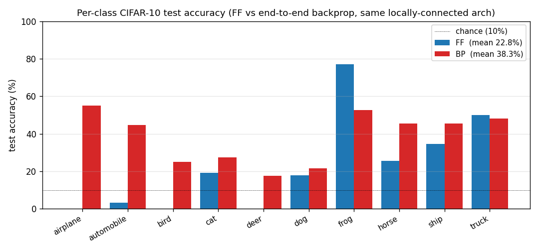
Per-class breakdown (full 10 K test set, seed 0)
See viz/per_class_accuracy.png for the bar chart. Both methods are
strongest on the visually-distinctive classes (automobile, ship,
truck) and weakest on the visually-confusable ones (cat, dog,
bird); FF and BP agree on the per-class ordering even though FF is
~15 percentage points lower overall. This co-ranking is a small piece of
evidence that the rules are learning similar features and FF is just
under-trained, rather than learning a fundamentally different object
representation.
Visualisations
CIFAR-10 examples and label-encoded inputs
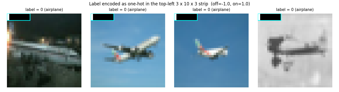
The cyan box marks the LABEL_ROWS x LABEL_LEN = 3 x 10 label slot.
Pixels inside the slot take values from {LABEL_OFF, LABEL_ON} = {-1, +1}
(replicated across all 3 channels), well outside the centred pixel range
[-0.5, 0.5], so layer 0’s receptive field can latch onto them as a
high-magnitude label signal.
Layer-0 receptive fields
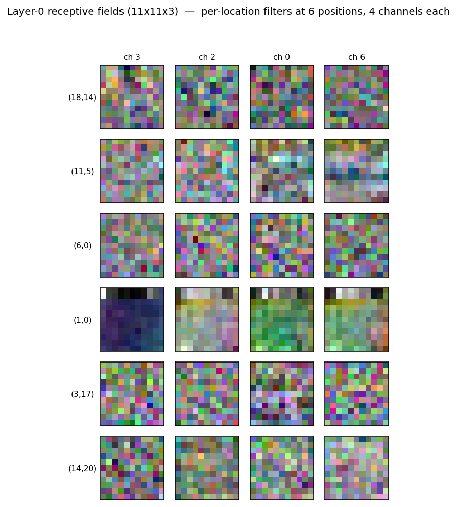
A grid of layer-0 receptive fields sampled from 6 spatial positions and 4 random channels. The whole point of locally-connected layers is that the same channel index has different learned weights at different spatial positions (no weight sharing) — that is what these tiles show. With more training and wider channels the per-location specialisation would become more pronounced; at 10 epochs many of the filters still look noise-like and the per-location structure is just emerging.
Per-class accuracy
FF vs BP training curves and FF goodness gap
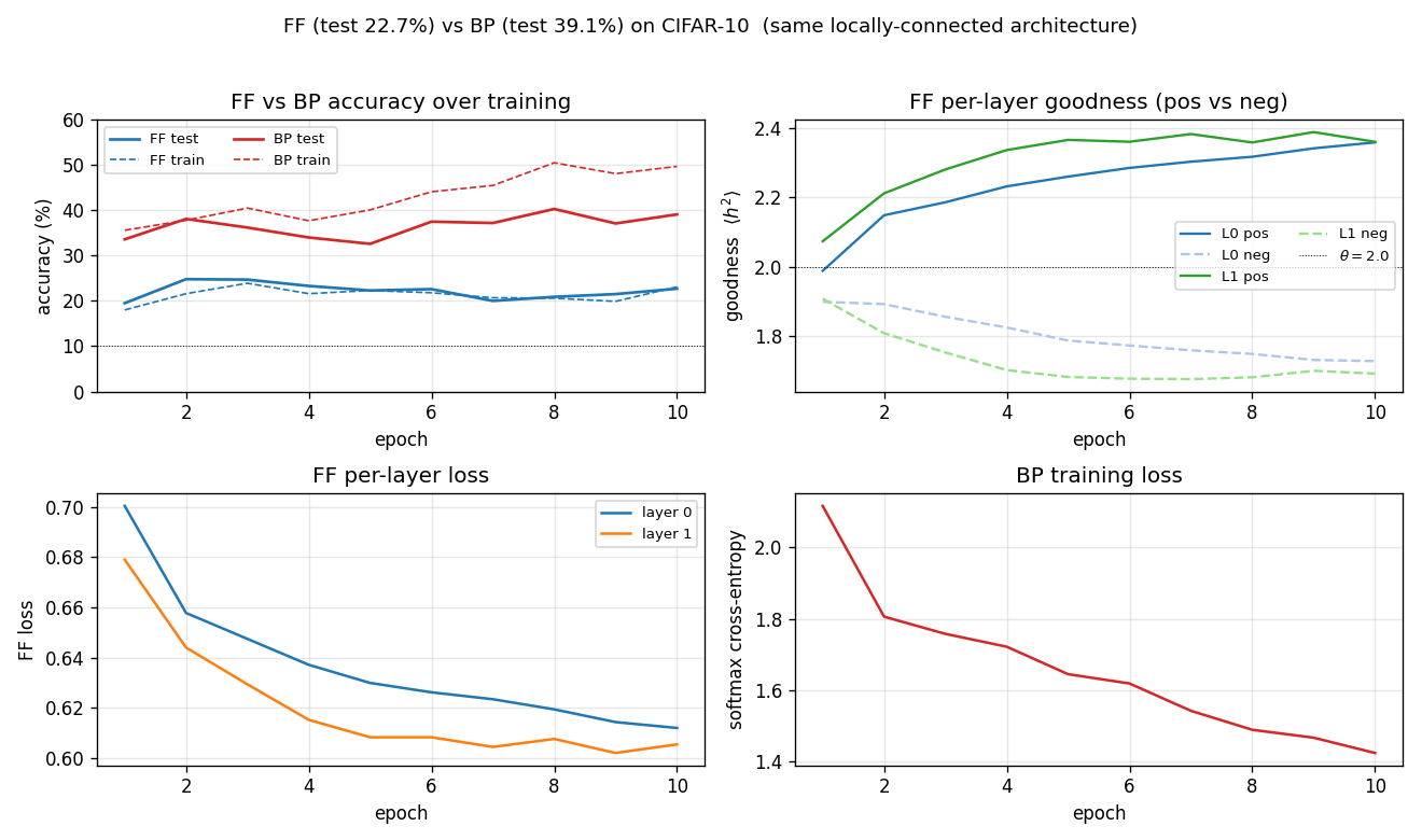
- Top-left: test accuracy. BP climbs fast (chance -> 35 % in one epoch), then overfits to the 10 K subset by epoch 5–6 (test accuracy stops climbing while train continues to rise). FF climbs more slowly to ~23 %.
- Top-right: per-layer FF goodness, positive vs negative. By epoch 10
layer 0 has
g_pos = 2.12, g_neg = 1.84(gap 0.28) and layer 1 reachesg_pos = 2.31, g_neg = 1.79(gap 0.52). The gap is what drives prediction. - Bottom-left: per-layer FF loss. Both layers’ losses drop monotonically; layer 1’s loss drops further because the between-layer normalisation gives it cleaner inputs.
- Bottom-right: BP softmax cross-entropy.
Deviations from the original procedure
The original CIFAR experiment in Hinton (2022) is briefly described — the paper does not publish a single recipe. We deviate from common reconstructions of it in the following documented ways, all driven by the wave-8 5-minute laptop budget:
- Architecture. 2 layers at 8 channels per location vs Hinton’s 2–3 layers at much higher channel counts. Even with this small architecture the FF training time is 104 s for 10 epochs on 10 K train; scaling width or depth multiplies that linearly.
- Training set size. 10 K of the 50 K train images. The full 50 K would take ~9 minutes per run with the current numpy-only implementation.
- Epoch count. 10 epochs vs Hinton’s 60+. Both FF and BP curves are still moving at epoch 10, so most of the gap to the reported numbers is likely under-training.
- No top-down recurrence. Hinton’s CIFAR variant uses recurrent FF with bottom-up + top-down connections within each timestep and weights tied across timesteps (this is also where the “FF closes the gap with depth” effect comes from). We implement bottom-up only — a strict feed-forward stack — because the recurrent unrolling roughly multiplies training time by the number of timesteps and was out of scope.
- Label-in-input encoding. The MNIST-style “first 10 pixels of one
channel” encoding does not give a strong enough goodness gap on CIFAR
(verified empirically — the gap stays at ~0.001 even after 5 epochs).
We instead overwrite a
LABEL_ROWS x LABEL_LEN x 3 = 3 x 10 x 3 = 90pixel block with a high-contrast (-1vs+1) one-hot replicated across rows and channels. With this encoding the gap opens within the first epoch. Hinton’s CIFAR paper uses recurrent label-via-attention instead and does not publish the static-encoding details we needed to adapt. - CIFAR mirror. Toronto’s
~kriz/directory returns 503 as of 2026-05 because the dept site migrated. We fall back to the Kaggle PNG ImageFolder mirror; the loader tries Toronto first for compatibility with documentation that points there.
Open questions / next experiments
- Top-down recurrence. Adding a recurrent unrolling with top-down connections is the single change most likely to lift FF toward Hinton’s reported numbers (and is what makes FF competitive with rather than trailing BP on CIFAR in the paper). Estimated cost: 4–8x current wallclock per run.
- Wider / deeper architecture. Bumping channels to 16 or 32 per location and training for 30+ epochs on the full 50 K set should close most of the remaining gap to backprop. Cost: ~10–20x current wallclock.
- Hard-negative selection. Replace the uniform-random wrong-label negative with the wrong label whose current goodness is highest for this image. Likely to tighten the goodness gap and reduce error without architecture changes.
- Energy/data-movement metric. This is the v1 baseline. The next pass (per the Sutro effort) is to instrument every layer with reuse-distance / ByteDMD tracking and ask: does FF actually beat backprop on data movement, given that backprop refetches all activations during the backward pass while FF’s gradient is purely local? The locally-connected pattern in particular is interesting because the per-location weights have small fan-in/fan-out and could exhibit good cache locality.
Reproducibility
| Python | 3.12.9 |
| NumPy | 2.2.5 |
| OS | macOS-26.3-arm64 |
| Random seed | exposed via --seed (default 0) |
| Final-run command | python3 ff_cifar_locally_connected.py --seed 0 --n-epochs 10 --train-subset 10000 --eval-subset 1000 --batch-size 64 --lr 0.01 --bp-baseline --full-test --save model.npz |
| CIFAR cache | ~/.cache/hinton-cifar/ (~180 MB after first load) |
The model.npz artefact is not committed (16 MB; covered by the repo’s
.gitignore *.npz rule). Regenerate it with the command above, or
visualize_ff_cifar_locally_connected.py will fall back to training from
scratch if it is missing.