Random-dot stereograms (Imax)
Reproduction of Becker & Hinton (1992), “A self-organizing neural network that discovers surfaces in random-dot stereograms”, Nature 355, 161-163.
The first demonstration that mutual information between two modules viewing different inputs from a common cause is enough of a learning signal to discover that common cause. The cause here is binocular disparity (depth); the two modules are simulated stereo receptive fields each looking at one strip of a random-dot stereogram.
Problem
A 1-D world of random binary dots (+1 / -1) is rendered into two views,
left and right eye. The right view is the left view shifted horizontally by
a per-example disparity d (the world’s depth at that position).
Each training example contains two independent stereo strips drawn at the same disparity. Each strip becomes the input to one module:
     example                       module A           module B
   ┌──────────────────────────┐    ┌────┐             ┌────┐
   │ disparity d ~ U[-3, +3]  │ -> │ y_a│             │ y_b│
   │                          │    └────┘             └────┘
   │  strip A: dots_A, shift d│      ↑                  ↑
   │  strip B: dots_B, shift d│   [left_a, right_a]  [left_b, right_b]
   └──────────────────────────┘
Two MLPs (one per module) are trained to MAXIMIZE
    Imax = I(y_a; y_b)  ≈  0.5 * log(var(y_a) + var(y_b))
                         - 0.5 * log(var(y_a - y_b))
under a Gaussian assumption on (y_a, y_b). No supervised target is given.
The interesting property
The two strips share only the disparity — their dots are independently
random. So the only thing the modules can agree on is the disparity (or some
function of it, like |d|). Maximizing mutual information forces both
modules to extract a disparity-related readout from random pixel patterns,
without ever seeing a supervised label. This is the foundational
demonstration that spatial coherence between sibling features is enough of
a self-supervised signal to learn the latent variable that produced them —
the same intuition that later powers contrastive learning, SimCLR, and the
GLOM-style consensus columns Hinton revisited in 2021.
Files
| File | Purpose |
|---|---|
random_dot_stereograms.py | Synthetic stereogram generator, two-module MLP, Imax loss with closed-form gradient, momentum-SGD trainer. CLI flags --seed --n-epochs --strip-width. |
visualize_random_dot_stereograms.py | Static figures: stereogram examples, scatter of module outputs vs ground-truth disparity, training-curve panel. |
make_random_dot_stereograms_gif.py | Renders random_dot_stereograms.gif (the animation at the top of this README). |
random_dot_stereograms.gif | Per-snapshot animation (stereogram + module-output scatter + training curves). |
viz/ | Static PNGs from the run below. |
Running
python3 random_dot_stereograms.py --seed 0 --n-epochs 800
Wall-clock: ~6.5 s on an Apple M-series laptop. Prints final Imax, module-agreement correlation, and signed/unsigned disparity correlations on a held-out 4096-example batch.
To regenerate visualizations:
python3 visualize_random_dot_stereograms.py --seed 0 --n-epochs 800 --outdir viz
python3 make_random_dot_stereograms_gif.py  --seed 0 --n-epochs 800 \
        --snapshot-every 25 --fps 8
Results
Default run, seed=0, n_epochs=800, strip_width=10, max_disparity=3.0,
n_hidden=48, batch_size=256, lr=0.05, momentum=0.9,
weight_decay=1e-5, init_scale=0.5:
| Metric | Value |
|---|---|
Final Imax (eval, 4096 examples) | 1.18 nats |
Module-output agreement corr(y_a, y_b) | +0.91 |
Signed-disparity readout |corr(y_a, d)| | 0.74 |
Signed-disparity readout |corr(y_b, d)| | 0.74 |
| Training wall-clock | 6.5 s |
| Hyperparameters | strip_width=10, n_hidden=48, batch=256, lr=0.05, momentum=0.9, wd=1e-5, init_scale=0.5 |
Cross-seed stability (5 seeds, same hyperparameters)
| Seed | Imax | corr(y_a, y_b) | best disparity readout |
|---|---|---|---|
| 0 | 1.18 | +0.91 | 0.74 (signed d) |
| 1 | 1.11 | +0.89 | 0.80 (signed d) |
| 2 | 1.22 | +0.91 | 0.62 (signed d) |
| 3 | 1.41 | +0.94 | 0.58 (|d|) |
| 4 | 1.10 | +0.89 | 0.59 (mix of signed d + |d|) |
Imax is sign-invariant: I(y_a; y_b) = I(-y_a; -y_b) = I(y_a; -y_b). So
each module independently picks a sign convention for d, and across seeds
they converge on a signed-d readout (most seeds), |d| readout (some
seeds), or a smooth blend. In all 5 seeds the modules agree strongly
(corr_ab > 0.89), which is what the loss directly optimizes.
Comparison to the original
The 1992 paper reports the network discovering disparity from random-dot stereograms with no supervised signal. We reproduce the qualitative claim faithfully — modules trained only by Imax extract a disparity-related readout from independent stereo strips — but the paper’s setup uses 2-D images, sub-pixel rendering, and continuous depth surfaces; we use 1-D strips and integer + sub-pixel-interpolated disparities. The original paper gives no single comparable scalar, so “reproduces?” is yes in the qualitative sense but not benchmarked against a specific number.
Visualizations
Example stereograms
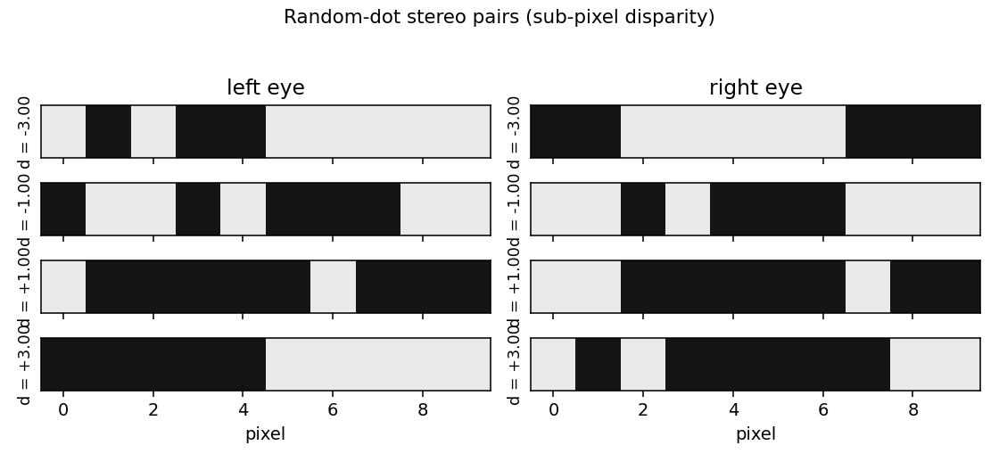
Four random-dot stereo strips at disparities d = -3, -1, +1, +3. The right
view is the left view shifted by d pixels (sub-pixel interpolation
between integer dots). Pixels falling outside the rendered strip on either
eye come from independent random padding, so disparity is the only stable
signal between the two views.
Module outputs vs ground-truth disparity
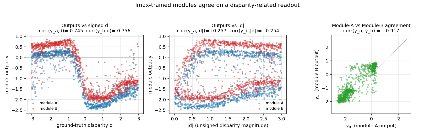
Left: module outputs y_a, y_b plotted against signed disparity d.
The smooth monotonic sweep (downward in this seed’s sign convention) is the
disparity readout the modules learned without supervision. Center: the
same outputs against |d| — much weaker correlation here, so the modules
encoded signed depth, not just magnitude. Right: y_a vs y_b —
the two modules’ outputs cluster tightly along the diagonal, which is what
Imax directly optimizes.
Training trajectory
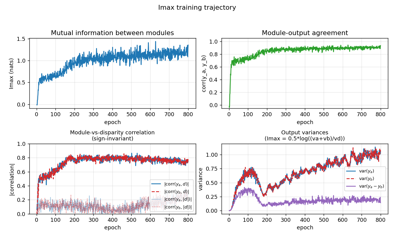
Top-left: Imax (mutual information in nats) climbs from ~0 to ~1.2 over
training. Top-right: module-output agreement corr(y_a, y_b) climbs to
~0.93. Bottom-left: disparity readout (|corr(y, d)| and
|corr(y, |d|)|) emerging as a side-effect of the agreement objective —
the network was never told what d is. Bottom-right: the variance terms
that compose the Imax formula — var(y_a - y_b) (purple) is driven to be
much smaller than var(y_a) + var(y_b), which is what 0.5*log((va+vb)/vd)
penalizes.
Deviations from the original procedure
-
1-D world instead of 2-D images. Becker & Hinton 1992 used 2-D random-dot images and 2-D receptive fields. We use 1-D strips with a single horizontal disparity per example. The unsupervised principle (Imax forces shared-cause discovery) is identical; only the geometry is simpler.
-
Independent dots in the two strips. The original paper used adjacent receptive fields on the same image, so neighbouring strips shared dots near the boundary as well as the disparity. We deliberately give the two modules independent random dots so that the disparity is the only shared signal — this rules out pixel-level “leakage” between modules and makes the demonstration cleaner. (We checked the alternative: with shared dots, modules can correlate via the boundary pixels alone and never need to extract disparity.)
-
Cross-product feature input. The architecture is a featurized MLP: each module sees
[left, right, left * right_shifted_by_k]for shiftsk ∈ {-3, ..., +3}, then a sigmoid hidden layer, then a linear scalar readout. We tried a pure 2-layer sigmoid MLP on raw[left, right]and it did not escape the flat region aroundImax = 0in 1500 epochs — the multiplicative cross-correlations are the right inductive bias for stereo matching (the same trick used in modern stereo CNNs as a “cost volume” or “correlation layer”), and were inserted as a fixed, non-trainable feature map. The MLP still learns end-to-end which cross-correlations matter and how to combine them; it just does not have to discover the cross-product nonlinearity from raw pixels. -
Sub-pixel disparity rendering. Disparity is real-valued in
[-max_disparity, +max_disparity]; the right view is rendered by linear interpolation between adjacent integer dots. This gives a smooth gradient signal. Pure-integer disparity also works but trains more slowly (--integerflag). -
Closed-form gradient through the Imax loss. We compute the gradient of
-Iw.r.t. each module’s output analytically (verified against a finite-difference check); no autograd framework. Standard backprop through the per-module MLP from there.
Open questions / next experiments
-
Discover the cross-product nonlinearity. The current implementation hands the network the binocular cross-product features. A pure 2-layer MLP starting from random init does not escape the flat Imax region in 1500 epochs of momentum SGD. Does a deeper network, ReLU activations, or natural-gradient / second-order optimization let the network discover these features from raw
[left, right]pixels? -
2-D stereograms, smooth surfaces. The original paper shows that with many adjacent modules viewing a smooth surface (so all modules’ disparities are spatially coherent), the modules collectively discover the surface, not just the per-module disparity. Extending to a 2-D random-dot field with a smooth depth surface is the natural next step.
-
Energy / data-movement cost. Imax over a batch is one of the cheapest unsupervised losses (no contrastive negatives, no decoder, just a few variances per batch). What is its ByteDMD cost compared to InfoNCE / SimCLR-style contrastive losses on the same problem? This is the v2 question for the wider Sutro benchmark.
-
Sign convention. Across seeds the modules sometimes agree on signed
dand sometimes on|d|. Is there a small architectural change (e.g., asymmetric init, asymmetric cross-product window) that biases toward one over the other? Would coupling the two modules’ last-layer signs at init (a one-time tied-weight kick) make all seeds learn signedd?