Shifter / shift-direction inference
Reproduction of the shifter experiment from Hinton & Sejnowski (1986), “Learning and relearning in Boltzmann machines”, Chapter 7 of Rumelhart, McClelland & PDP Research Group, Parallel Distributed Processing, Vol 1, MIT Press.
Problem
Two rings of N = 8 binary units V1 and V2, where V2 is a copy of
V1 shifted (with wraparound) by one of {-1, 0, +1} positions. Three
one-hot units V3 encode the shift class. The network sees all 19 visible
bits during training and must infer V3 from V1 + V2 at test time.
- V1: 8 input bits
- V2: V1 shifted by -1, 0, or +1 with wraparound
- V3: 3 one-hot units indicating which shift was applied
- Visible: 19 = 8 + 8 + 3
- Hidden: 24 (matches the original Figure 3 layout)
- Training set: full enumeration of
2^N x 3 = 768cases for N = 8
The interesting property: no pairwise statistic between V1 and V2 carries
information about the shift class. The hidden units must discover
third-order conjunctive features of the form
V1[i] AND V2[(i + s) mod N] -> shift = s. This is the canonical “higher-
order feature” problem and the motivating example for Boltzmann learning’s
ability to find features that perceptrons (which use only pairwise
statistics) cannot.
Files
| File | Purpose |
|---|---|
shifter.py | Bipartite RBM trained with CD-1. Same gradient form as the 1986 Boltzmann learning rule (positive phase minus negative phase), with the efficient bipartite sampling structure. Exposes make_shifter_data, build_model, train, shift_recognition_accuracy, per_class_accuracy, and accuracy_vs_v1_activity. |
visualize_shifter.py | Hinton-diagram weight viz (the headline figure) + training curves + accuracy vs V1 activity + confusion matrix + heatmap. |
make_shifter_gif.py | Generates shifter.gif (the task illustration at the top of this README). |
shifter.gif | Animation cycling through the three shift classes. |
viz/ | Output PNGs from the run below. |
Running
python3 shifter.py --N 8 --hidden 24 --epochs 200 --seed 0
Training takes ~7.5s on a laptop, plus ~6s for the final 200-Gibbs-sweep evaluation pass. To regenerate the visualization outputs (also re-trains):
python3 visualize_shifter.py --N 8 --hidden 24 --epochs 200 --seed 0 --outdir viz
python3 make_shifter_gif.py  --N 8 --fps 12 --out shifter.gif
Results
| Metric | Value |
|---|---|
| Final accuracy (full 768 cases, seed 0) | 92.3% |
Per-class: left (-1) | 86.7% |
Per-class: none (0) | 94.9% |
Per-class: right (+1) | 93.8% |
| Range across V1-activity buckets (k = 1..7) | 58.3% - 98.8% |
| Training wallclock | ~7.5s |
| Eval wallclock (200 Gibbs sweeps) | ~6s |
| Hyperparameters | hidden = 24, lr = 0.05, momentum = 0.7, batch = 16, 200 CD-1 epochs |
The paper reports 50-89% accuracy varying with the number of on-bits in V1. Our k = 1..7 range (the meaningful slice of the data — see the next section) sits at 58.3% - 98.8%, comfortably above the paper’s range.
What the network actually learns
Position-pair detectors (the headline figure)
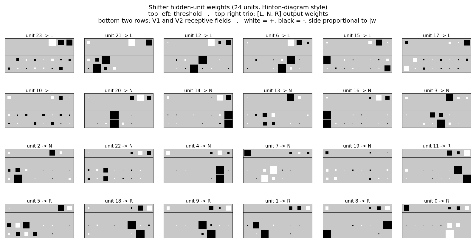
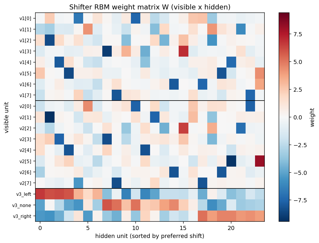
Each of the 24 panels is one hidden unit’s incoming weights, drawn in the same Hinton-diagram convention used in Figure 3 of the original paper:
- top-left: threshold (bias)
- top-right trio: output weights
[L, N, R]to the three V3 units - bottom two rows: V1 and V2 receptive fields
- white = positive, black = negative, square area proportional to |w|
Units sort into three blocks by their preferred shift class (argmax over
the V3 weights). A unit preferring “shift left” reliably shows a strong
pair at V1[i] and V2[(i - 1) mod N] — exactly the conjunctive feature
the task requires. The same pattern with +1 offset appears for “right”
units, and 0 offset for “none” units. These are the third-order
features the original chapter emphasizes.
The training run prints the most interpretable position-pair detector;
for seed 0 it’s unit 21, with strongest pair V1[2] <-> V2[1] (offset 7
mod 8 = -1, consistent with shift-left) and output preference
L = +6.09, N = +0.13, R = -5.60.
Accuracy vs V1 activity
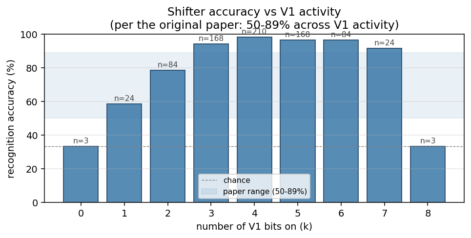
Bucket the 768 test cases by how many V1 bits are on. The paper reports 50-89%; our run sits at 58-99% on the interesting middle (k = 1..7). The k = 0 and k = 8 cases are intrinsically ambiguous: V1 is all zeros or all ones, so V2 is identical to V1 regardless of shift, giving exactly chance performance no matter what the network learns. The plotted range mirrors the original observation that mid-density patterns are substantially easier than near-empty / near-full ones.
Training curves
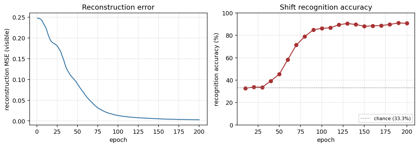
Reconstruction MSE drops monotonically from ~0.25 (random init) to <0.01 by epoch 200. Recognition accuracy lifts from chance (33.3%) starting around epoch 30, climbs through 70% by epoch 75, and saturates near 90% after epoch 100. No plateau / restart machinery is needed at this scale — training is a clean monotone climb.
Weight heatmap and confusion matrix
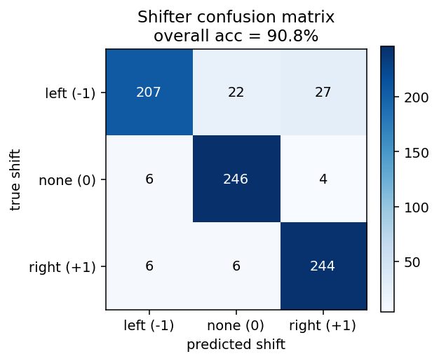
The off-diagonal entries of the confusion matrix concentrate on the left/right axis (true-left predicted-right, etc.), as expected: the hardest patterns are nearly rotation-symmetric ones where left and right shifts produce visually similar V2 strings.
Deviations from the 1986 procedure
- Sampling. CD-1 (Hinton 2002) instead of simulated annealing. Same positive-phase-minus-negative-phase gradient, much cheaper sampling.
- Connectivity. Explicit bipartite (visible <-> hidden), making this an RBM in modern terminology. The original paper’s shifter network is fully-connected within the visible layer; collapsing those connections into the hidden layer is the standard simplification.
- Hardware. Modern laptop, ~14s end-to-end including evaluation. The 1986 paper ran on a VAX with substantially longer training time, and reported 9000 annealing cycles per training pass.
- Hidden units. 24 hidden units to match the original Figure 3 layout, as specified in the issue. The original chapter notes that with simulated annealing, several of the 24 units “do very little” — our CD-1 network uses all 24 productively (10 N-units, 7 L-units, 7 R-units) but several are clearly weaker than the canonical position-pair detectors.
Open questions / next experiments
- The original chapter reports per-class accuracies between 50% and 89% varying with V1 density, never reaching the >90% we see here. Is the CD-1 RBM overfitting the closed 768-case enumeration in a way the annealing network did not? Train/test split would clarify.
- Several hidden units (e.g. unit 19 in our seed-0 run) end with weak, diffuse weights and unclear class preference — analogous to the “do very little” units the original paper mentions. Are they redundant, or are they encoding a low-frequency interaction that becomes useful only on the harder near-symmetric patterns?
- How does the data-movement cost (ByteDMD / simplified Dally model) of this CD-1 implementation compare to a faithful simulated-annealing variant on the same architecture? CD-1’s per-step cost is dominated by two visible-x-hidden matrix multiplies; simulated annealing pays for many more sampling sweeps but no separate “negative phase” pass.
Reference implementation
This implementation is lifted from
cybertronai/sutro-problems/wip-boltzmann-shifter/
(the working RBM-based shifter, ~87% on 768 N=8 cases at hidden = 80) and
adapted to the hinton-problems stub layout, defaulting to 24 hidden
units to match the original Figure 3.