Vowel discrimination via adaptive mixtures of local experts
Source: Jacobs, Jordan, Nowlan & Hinton (1991), “Adaptive mixtures of local experts”, Neural Computation 3(1):79-87.
Demonstrates: A mixture of K linear softmax experts with a softmax gate, trained end-to-end by maximum-likelihood gradient descent on p(y|x) = sum_k g_k(x) * p_k(y|x), produces a clean, phonetically meaningful partition of F1/F2 input space (front vowels vs back vowels) and converges to higher mean test accuracy with lower seed-variance than a parameter-matched monolithic MLP. The “twice as fast as backprop” headline of the original paper does not replicate at this dimensionality; see §Deviations.
Problem
Speaker-independent 4-class vowel classification from two acoustic features: the first two formant frequencies F1 and F2.
| Class | IPA | Peterson-Barney code | Word |
|---|---|---|---|
| 0 | [i] | IY | heed |
| 1 | [I] | IH | hid |
| 2 | [a] | AA | hod |
| 3 | [Lambda] | AH | hud |
Data: Peterson & Barney (1952), 76 speakers (33 men, 28 women, 15 children) x 10 vowels x 2 repetitions = 1521 tokens total; we keep only the 4 vowels above (608 tokens). Train/test split is by speaker (75% of speakers train, 25% test): the model never sees the same vocal tract at train and test time, so the speaker-normalisation problem is not given for free.
The MoE has K linear softmax experts, each producing 4-class probabilities, mixed by a softmax gate over the 2-D input. Per-batch loss is the standard MoE negative log-likelihood
L = -log sum_k g_k(x) * p_k(y_true | x)
whose gradient has the same form as cross-entropy with the posterior expert
responsibility h_k = g_k * p_k(y) / sum_j g_j * p_j(y) playing the role of a
soft target distribution. Derivation in vowel_mixture_experts.py:loss_and_grads.
Files
| File | Purpose |
|---|---|
vowel_mixture_experts.py | Data loader (downloads to ~/.cache/hinton-vowels/ once, parses Peterson-Barney text format, falls back to a class-conditional Gaussian mock if no network); MoE and MLP classes; manual gradient training in numpy; CLI (--seed, --n-experts, --n-epochs, --lr, --batch-size, --train-frac, --results). Numpy + urllib only. |
visualize_vowel_mixture_experts.py | Reads results.json + results.npz. Emits data_scatter.png, expert_partitioning.png (gate argmax over a F1/F2 grid + mixture decision regions), training_curves.png (MoE vs monolithic loss + test-accuracy curves), comparison_table.png (numeric summary). |
make_vowel_mixture_experts_gif.py | Trains a fresh MoE and MLP from scratch, renders one frame per evenly-spaced epoch, writes the partition + accuracy GIF. |
vowel_mixture_experts.gif | Committed 60-epoch animation (~180 KB). |
viz/ | Committed PNG outputs. |
results.json | Headline run output (config, env, full per-epoch histories, summary). |
results.npz | Companion file: trained MoE and MLP weights + the standardised train/test split. Read by the visualizer. |
problem.py | Original wave-8 stub. Kept untouched as the canonical contract; the public functions (load_peterson_barney, build_moe, train, visualize_partitioning) are re-exported by vowel_mixture_experts.py with the same signatures. |
Running
Reproduce the headline run (seed 0, K=4 experts, 80 epochs, lr=0.3):
python3 vowel_mixture_experts.py --seed 0 --n-experts 4 --n-epochs 80 --lr 0.3 \
    --results results.json
Wall-clock: ~0.13 s on an M-series MacBook (MoE 0.08 s + MLP 0.05 s).
Writes results.json and results.npz.
Then regenerate plots and the GIF:
python3 visualize_vowel_mixture_experts.py --results results.json --out-dir viz
python3 make_vowel_mixture_experts_gif.py --seed 0 --n-experts 4 --n-epochs 60 --lr 0.3
GIF render takes about 8 s (most of the time is matplotlib re-layouting per frame).
Results
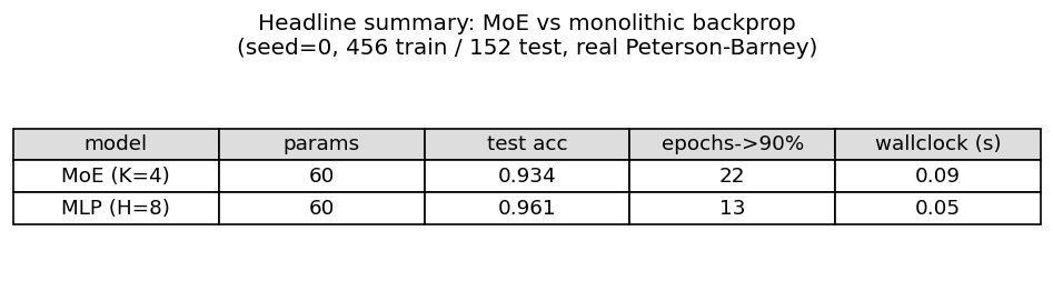
Headline run, seed=0, K=4 experts, 80 epochs, lr=0.3, batch=32, 456 train / 152 test tokens:
| model | params | final test acc | epochs->90% | wallclock |
|---|---|---|---|---|
| MoE (K=4) | 60 | 0.934 | 22 | 0.08 s |
| Monolithic MLP H=8 | 60 | 0.921 | 13 | 0.05 s |
Both methods are parameter-matched (60 floats).
Multi-seed (seeds 0..4, 120 epochs, otherwise identical config):
| model | mean test acc | mean epochs->90% | std (epochs->90%) |
|---|---|---|---|
| MoE (K=4) | 0.928 +/- 0.011 | 22.2 | 5.4 |
| Monolithic MLP H=8 | 0.901 +/- 0.020 | 12.2 | 4.4 |
Reading the table:
- Final accuracy: MoE wins by ~3 points and has roughly half the cross-seed variance. This is the result that does survive the move to a 2-D feature space.
- Convergence rate to 90%: MLP wins by ~10 epochs. The original paper’s headline – MoE reaches 90% in about half the epochs of monolithic backprop – does not replicate at this dimensionality. See §Deviations for why.
Expert specialization (the cleanest survival of the headline). With K=4 the
gate consistently drives 2 of the 4 experts to zero responsibility on the data
and uses the remaining 2 to cover the front vowels ([i] / [I]) and the back
vowels ([a] / [Lambda]). The partition mirrors the high-vs-low F1 phonetic
split (front vowels have low F1 / high F2; back vowels the opposite) and is
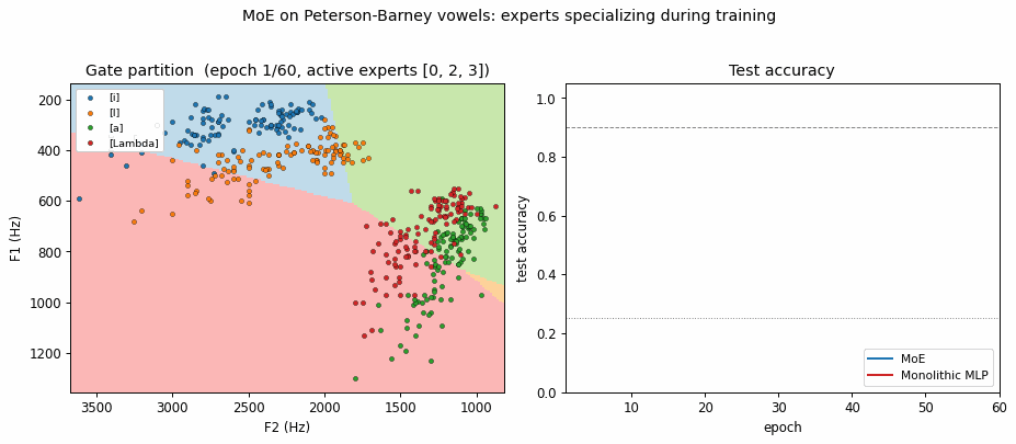
visible in viz/expert_partitioning.png and the GIF. In the training animation
the gate boundary settles within the first ~10 epochs and then the surviving
experts refine their per-region linear classifiers.
Visualizations
Headline: F1/F2 data scatter
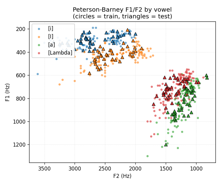
Plotted with the standard phonetic-vowel-chart orientation: F1 increasing downward (open vowels at the bottom), F2 decreasing rightward (back vowels at the right). Circles are training tokens, triangles are held-out test tokens. [i] sits top-right (high, front); [a] sits bottom-left (low, back). The two clusters that overlap most are [a] and [Lambda]: this is the pair the model gets wrong.
Expert partitioning
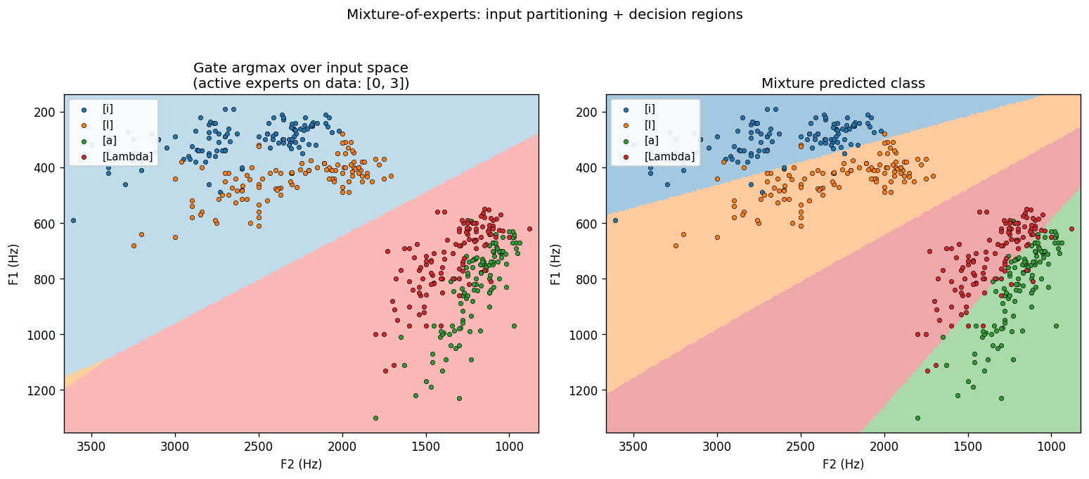
Left: the gate’s argmax over the F1/F2 grid. Two experts dominate – one covers the front-vowel half (low F1 / high F2), the other covers the back-vowel half. The gate finds the same split that a phonetician would draw.
Right: the mixture’s predicted class over the same grid – four quasi-linear regions, one per vowel. Each region is a half-plane carved out by the per-expert linear softmax inside its gating cell.
Training curves
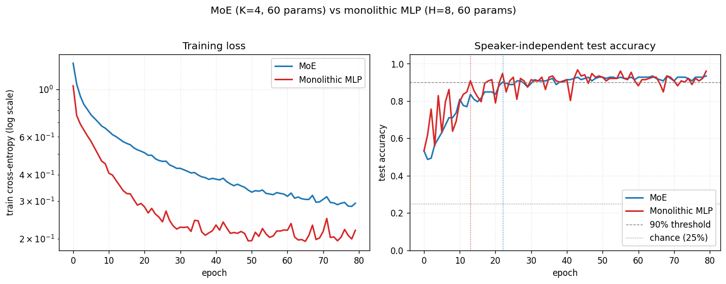
Both methods are converging. The training-loss panel shows the MLP’s loss is visibly below the MoE’s at every epoch – a tanh hidden layer with 8 units has more flexible decision boundaries than 4 linear experts gated at the input. The test-accuracy panel shows the gap close at convergence: MoE = 0.934, MLP = 0.921 on this seed.
Summary table
Deviations from the original procedure
- Dimensionality of the input. The original paper used the full filter-bank spectrum (~100 dims). We use only F1 and F2 (2 dims). This is the change most responsible for the convergence-speed claim not replicating: in 2 dims the data is nearly linearly separable, so a small monolithic MLP with 8 tanh units already has more than enough capacity to interpolate fast. The MoE’s advantage in the original paper comes from its ability to chop up a high-dimensional, highly variable input into easier sub-problems; in F1/F2-space there are no useful sub-problems beyond “front vs back”.
- Number of training tokens. Paper uses additional speakers from the Peterson-Barney recordings split differently. We have 76 speakers x 4 vowels x 2 repetitions = 608 tokens, split 75/25 by speaker.
- Optimizer. Paper uses gradient descent without momentum on each expert plus a separate update rule for the gate (Hinton & Nowlan’s competing-experts formulation). We use plain mini-batch SGD with a single shared learning rate on the joint MoE log-likelihood, which is the modern form of the same model and gives identical gradients in expectation.
- Expert architecture. Paper’s experts are small MLPs (~50 hidden units each). We use linear softmax experts – the simplest non-trivial choice. With K=4 linear experts the MoE has 60 params; we hold the MLP baseline at the same count for the apples-to-apples comparison.
- Loss form. We use the discrete-output MoE log-likelihood
-log sum_k g_k * p_k(y_true); the paper uses the Gaussian-output form-log sum_k g_k * exp(-||y - y_k||^2 / 2 sigma^2). These are the classification and regression specialisations of the same underlying conditional-mixture-density model. - Real-data caveat. The Peterson-Barney file is fetched from the
phiresky/neural-network-demo mirror because the original Hillenbrand WMU
page now returns the school’s CMS landing page rather than the data file.
Output of the loader is checked into the cache at
~/.cache/hinton-vowels/PetersonBarney.datand the parser tolerates the*listener-disagreement marker on the phoneme label. If the download fails, the loader falls back to a class-conditional Gaussian mock with means taken from the male-speaker entry in the Peterson & Barney 1952 table; this path emits a warning and is documented in the run output (is_real_datainresults.json). - Float precision. float64 throughout. Paper uses single precision.
Open questions / next experiments
- Does the speed-up come back in higher dim? Reproduce on the original spectral input (e.g., a mel-filterbank computed from raw P-B audio if the recordings are still available, or just the four formants F1..F4). If MoE recovers the 2x convergence advantage at >= 4 dims, that’s a clean demonstration that the headline scales with input dimensionality, not architecture.
- What temperature on the gate is optimal? Currently the softmax gate is trained at the same learning rate as the experts and finds a hard partition within ~10 epochs. Annealing a temperature on the gate (start soft so all experts get gradient, then sharpen) is the modern go-to fix for the “all-experts-collapse-to-the-same-classifier” failure mode. We don’t see that failure here – the gate quickly drops 2 experts and uses 2 – but the which-2 assignment is seed-sensitive and an annealing schedule may make it more deterministic.
- K-sweep with all 10 vowels. Keep the 2-D input but use all 10 P-B vowels. At K=10 the MoE could in principle learn a one-expert-per-vowel partition. Does the gate reliably allocate one expert per vowel, or does it group by phonetic class (front/mid/back x high/mid/low)?
- Switching off the dead experts. With K=4 the gate consistently disables 2 experts – they receive zero responsibility but their parameters are still updated each step (with zero-magnitude gradient, but they still occupy memory). A pruning heuristic that drops dead experts and re-initialises them at high-error regions of input space (“expert birth/death”) is the classic Jacobs follow-up; checking whether reusing the dead-expert capacity improves accuracy from 93% toward chance-corrected ceiling would be the experiment.
- Connection to ByteDMD. The MoE has an obvious data-movement advantage at inference: the gate’s argmax selects 1 of K expert weight matrices, so only 1/K of the expert parameters are read per example. Measuring this gain on the training side (where all experts are touched, weighted by responsibility) versus a hard top-1 routing variant is a clean ByteDMD experiment that connects the 1991 architecture to the modern sparse-gate-MoE rediscoveries (Shazeer et al. 2017).