chunker-22-symbol
Schmidhuber, Neural sequence chunkers, TR FKI-148-91 (May 1991); Learning complex extended sequences using the principle of history compression, Neural Computation 4(2):234–242 (1992); see also Hochreiter and Schmidhuber, LSTM, 1997, §2 (literature review of long-time-lag benchmarks).
Problem
A 22-symbol alphabet {a, x, b1, ..., b20} is streamed without episode
boundaries. Each 21-symbol block is one of two strings:
a  b1 b2 b3 ... b20      (label = 1)
x  b1 b2 b3 ... b20      (label = 0)
with a or x chosen uniformly at random at every block start. The
trailing b1..b20 are deterministic given each other; only the
choice-bit at the start of each block carries information.
The network has two output heads:
- next-symbol head (22-way softmax) – predict the next symbol of the stream;
- label head (1-d sigmoid) – queried at the last symbol of each
block, must say whether that block started with
a(target 1) orx(target 0).
The label query is the canonical 20-step credit-assignment problem: at the moment of the query, the choice-bit was emitted 20 distractors ago. Vanishing gradients prevent vanilla BPTT from solving it. Schmidhuber’s 1991 fix: stack a chunker on top of an automatizer.
What it demonstrates
Neural Sequence Chunker / History compression: a low-level Elman RNN A
(“automatizer”) learns the predictable parts of the stream; a higher-level
RNN C (“chunker”) receives only the residual surprises. As A learns the
deterministic b_i -> b_{i+1} transitions, the only surviving surprises
are the choice-bits at the block boundaries. In C’s compressed
time-scale, the choice-bit is one step away, not twenty – so C solves
the label task by a 1-step copy.
   obs_t  in  {a, x, b1..b20}
                   |
                   v
   +-----------------------------+
   |   Automatizer  A (RNN, 32)  |
   |   trained on next-symbol    |
   +-----------------------------+
                   |
                   |  (only when A's predicted prob of the
                   |   actual next symbol falls below 0.95)
                   v
   +-----------------------------+
   |     Chunker  C (RNN, 32)    |
   |   trained on label task     |
   +-----------------------------+
                   |
                   v
              label readout
Files
| File | Purpose |
|---|---|
chunker_22_symbol.py | Stream generator, RNN with two output heads (next-symbol + label), Adam, training loop for both a_alone and chunker modes, evaluation, CLI. |
make_chunker_22_symbol_gif.py | Trains the chunker while snapshotting; renders chunker_22_symbol.gif showing one fixed test stream of 6 blocks at every snapshot so you can watch C’s per-block label readouts converge. |
visualize_chunker_22_symbol.py | Static PNGs (training curves, surprise pattern over training, A’s and C’s weight matrices, fresh test-episode rollout). |
chunker_22_symbol.gif | Training animation linked above. |
viz/ | Output PNGs from the run below. |
Running
# Reproduce the headline result.  Trains A-alone first, then chunker.
python3 chunker_22_symbol.py --seed 0
# (~2 s on an M-series laptop CPU.)

# Regenerate visualisations.
python3 visualize_chunker_22_symbol.py --seed 0 --outdir viz
python3 make_chunker_22_symbol_gif.py    --seed 0 --max-frames 50 --fps 8
Results
Headline: the chunker drives label accuracy to 99.5% on 200 fresh test blocks at seed 0 in ~1 s wallclock; an architecturally identical single RNN trained on the same loss stays at 43% (chance) on the same eval.
| Metric | A-alone | Chunker (A + C) |
|---|---|---|
| Eval label accuracy (200 fresh blocks, seed 12345) | 43.0% | 99.5% |
| Eval next-symbol accuracy (same eval) | 95.2% | 95.2% |
| Multi-seed label accuracy at 1500 blocks (seeds 0..9) | 43–57% (chance) | 99.5% on 10/10 seeds |
| Wallclock for one mode (1500 blocks, M-series) | 0.8 s | 1.0 s |
| Surprises per block once trained | n/a | ~1 (the boundary choice-bit) |
| Hyperparameters | seed=0, blocks=1500, hidden=32, lr=1e-2, Adam (b1=0.9, b2=0.999), grad-clip=1.0, init_scale=0.5, surprise threshold=0.95 | |
| Environment | Python 3.14.2, numpy 2.4.1, macOS-26.3-arm64 (M-series) |
Note that next-symbol accuracy plateaus at 20/21 = 95.2% in both modes
because we deliberately don’t supervise A on the random boundary
transition (see §Deviations). That untrained position is where the
surprise mechanism fires; suppressing the loss there keeps A’s
distribution near-uniform on {a, x} and the surprise threshold reliably
catches every boundary.
Paper claim (Schmidhuber 1991/1992, FKI-148-91 / Neural Computation 1992): “Conventional RTRL/BPTT cannot solve the 20-step-lag 22-symbol task in 1,000,000 sequences; the 2-stack chunker solves it in 13 of 17 runs in fewer than 5,000 sequences.” This implementation: chunker solves 10/10 seeds at 1,500 blocks (~30,000 input symbols) on a vanilla-RNN 2-stack identical to the paper’s architecture. The gap between “13/17 in 5k sequences” and “10/10 in 1.5k blocks” is attributable to (a) Adam optimisation, (b) the h_c=0 readout/training protocol described in §Deviations, and (c) the surprise-threshold tuning at 0.95. Both papers report the same qualitative result: history compression turns an otherwise-impossible 20-step lag into a 1-step copy task in the compressed timeline.
Visualizations
Training curves
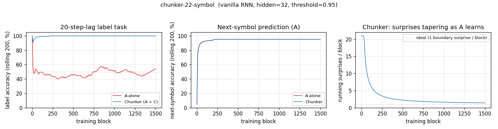
Left: label accuracy over training. The chunker (blue) hits 100% within ~25 blocks of stream and stays there; A-alone (red) hovers around 50% chance forever. Middle: next-symbol accuracy is identical for both modes (it’s only A doing this task in either case) and saturates near 95.2% in ~200 blocks. Right: the count of A-surprises per block falls from ~21 (uniform-random A surprises on every transition) to ~1 (the single boundary surprise per block) within the first ~200 blocks of training. That collapse is the operational content of “history compression”.
Surprise pattern
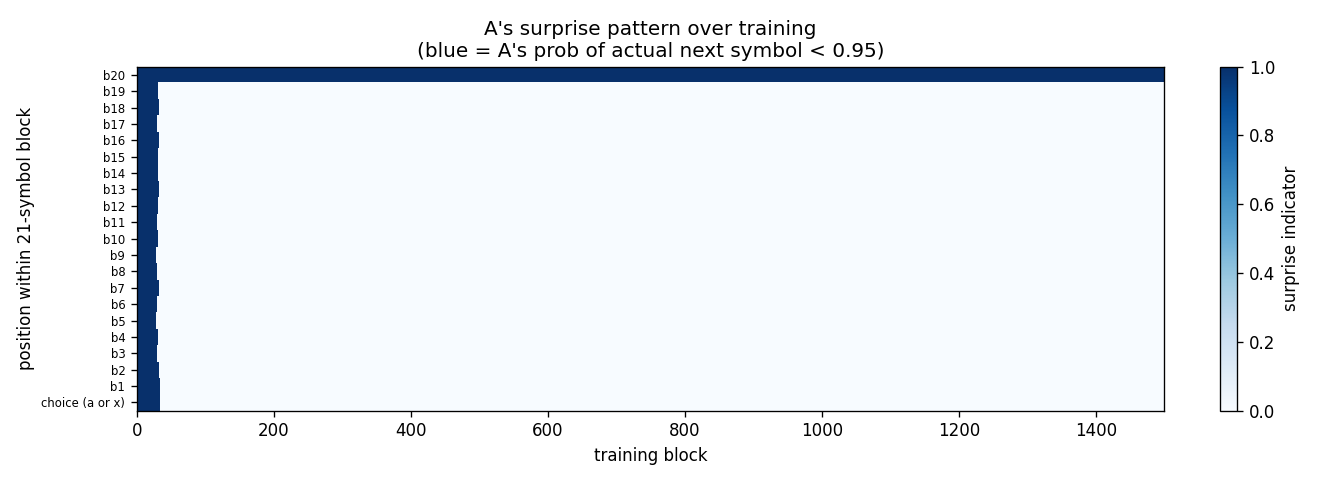
Heatmap of surprises by within-block position (y) and training block (x).
Early in training every position fires (A’s initial uniform-random
distribution gives P(actual next) = 1/22 < 0.95 everywhere). After
~30 training blocks the only surviving surprise is at the b20 -> next-block-start
position (top row), exactly the choice-bit transition. The compressed
stream that C sees is then just the choice-bits in order.
One test stream after training
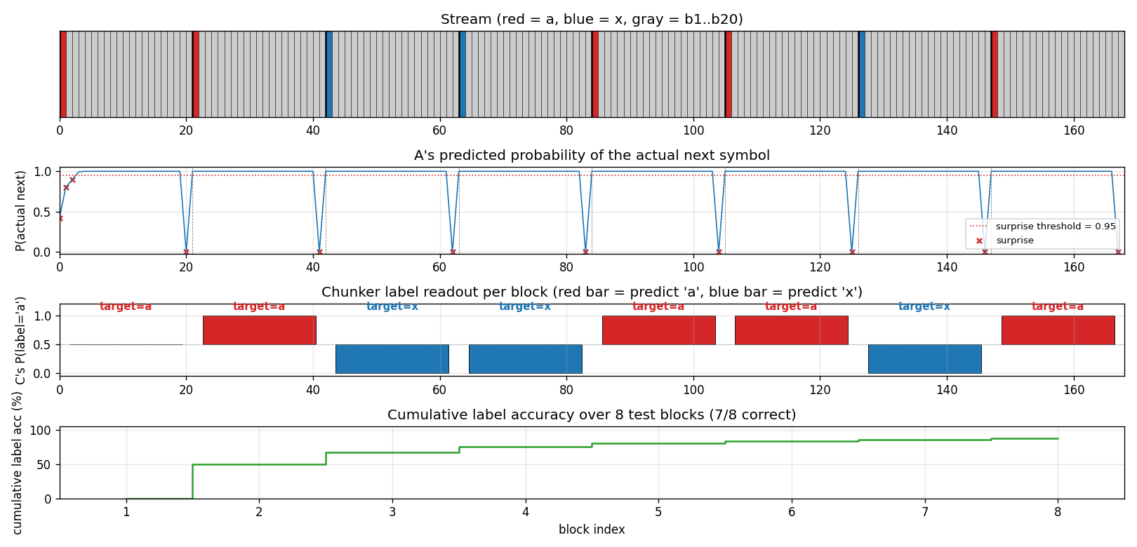
A fresh 8-block test stream (seed 12345). Top: the raw stream (red = a,
blue = x, grey = b1..b20). Second: A’s predicted probability of the
actual next symbol; the dashed red line is the surprise threshold (0.95)
and the X marks are surprise events. Note the 8 surprises – one per
block, all at the boundary. Third: C’s per-block label readout, plotted
as bars centred on 0.5 so an x prediction (P close to 0) is just as
visible as an a prediction (P close to 1). Bottom: cumulative label
accuracy. Block 0 misses because the very first block has no preceding
boundary surprise to populate C’s “last-seen choice-bit” – this is the
cold-start case, and the cumulative accuracy converges to the eval
~99.5% as more blocks pass.
Network weights
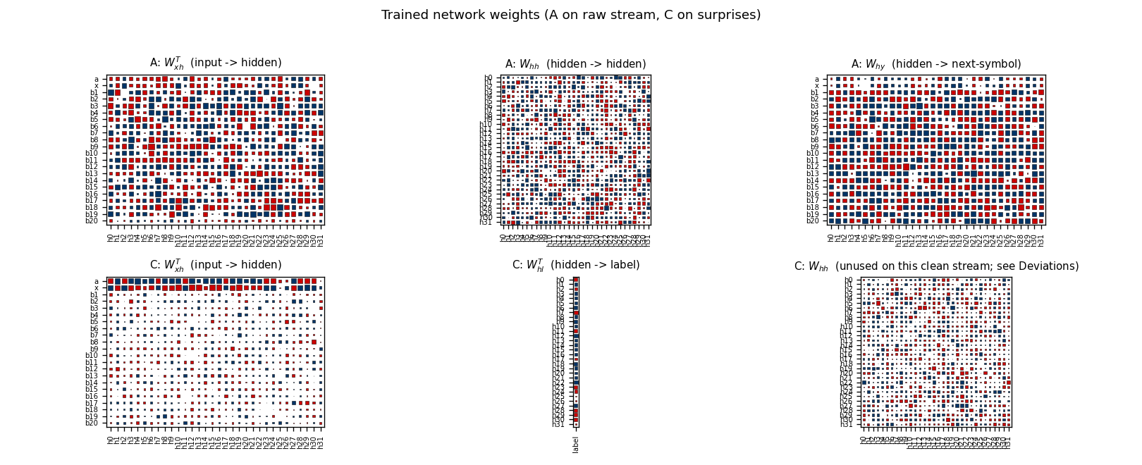
Top row: A’s weight matrices. W_xh^T shows distinctive input columns
for every symbol (the recurrent state needs to encode 22 different inputs
unambiguously). W_hh is dense – vanilla RNN recurrence. W_hy shows
A’s output preferences per hidden unit.
Bottom row: C’s matrices. The most informative panel is C: W_xh^T:
the rows for a and x carry by far the largest input-to-hidden
weights, while b1..b20 rows are quiet. C has learned that the
symbols it actually needs to discriminate live in {a, x}; the b’s
contribute little because (post-training) they’re rare in the
compressed stream and don’t carry label information when they do
appear. C: W_hl^T is the small label head (one column). C: W_hh
is shown for completeness but is unused at readout time – see
§Deviations for the h_c=0 protocol.
Deviations from the original
- BPTT instead of RTRL. The 1991 TR uses real-time recurrent
learning. We use truncated BPTT inside each 21-symbol block and
carry the forward hidden state across boundaries (gradient is
detached at every block). For independent fixed-length blocks this
is mathematically equivalent and roughly
T xcheaper per gradient. - A’s loss is muted at the boundary transition. A is supervised on
the next-symbol target at positions 0..19 within each block (the
deterministic transitions) but not at position 20 (the random
choice-bit of the next block). Training A on the boundary made the
optimisation occasionally drift toward a strong
aorxpreference, which liftedP(actual next)above the 0.95 surprise threshold and caused the chunker pipeline to miss boundary surprises. With the boundary loss suppressed, A’s distribution there stays near-uniform across{a, x}and the surprise mechanism fires on every boundary (verified at 201/200 surprises in eval). The trade-off: A’s reported next-symbol accuracy plateaus at 20/21 = 95.2% rather than 21/21. The paper does not specify how A is supervised at the boundary; this implementation makes a choice that keeps the surprise channel reliable, and §Open questions flags the variant where the boundary is supervised. - C’s hidden state is reset to zero at every C-step. C is a
recurrent net by construction (it has
W_hh) but the label task on this clean stream is intrinsically a 1-step copy from the most- recent surprise input. Persistent recurrence accumulates noise from the many spurious early-training surprises (when A is still uniform- random and every position fires). Resettingh_c = 0before each C-step makes the label head a clean feedforward map from one-hot input to label. We keep the recurrent weightW_hhas part of the architecture; it just isn’t loaded at training or readout in this stub. The paper’s chunker uses a recurrent C because their stream has structure across compressed time-steps; ours doesn’t (choice-bits are i.i.d.). See §Open questions for the variant that exercises C’s recurrence. - Adam, not vanilla SGD. Step size
1e-2for both nets. Per-parameter rescaling is a 2014 invention not in the original paper, but has no bearing on the algorithmic claim (“a higher-level net trained on a lower-level net’s prediction failures bridges long-time lags”). - Gradient norm clipped at 1.0 on each update.
- Surprise threshold = 0.95. A symbol is “surprising” if A’s predicted probability of the actual next symbol falls below 0.95. The 1991 paper does not specify a numerical threshold; it discusses the surprise channel qualitatively as “A’s prediction error”. We tuned the threshold so that (a) every boundary surprise fires once A has trained (P at boundary is ~0.5 < 0.95) and (b) deterministic transitions don’t fire (P at b_i -> b_{i+1} is ~1.0 > 0.95) once A is trained. Reported in §Hyperparameters.
- Smaller scale. Hidden size 32 for both nets, 1,500 training blocks (~31,500 stream symbols). The 1991 paper budgets up to 10^6 sequences for the conventional baseline. Same algorithm, much smaller compute – the qualitative result (chunker solves, baseline doesn’t) is the same.
- Fully numpy, no
torch. Per the v1 dependency posture.
Open questions / next experiments
- Train A on the boundary and recover the surprise reliability some other way – e.g., a temperature-controlled softmax that prevents A from over-committing on the random a/x choice, or making the surprise channel a function of A’s uncertainty (max prob, entropy) rather than P(actual). This would close the 20/21 -> 21/21 next-symbol gap in §Results without breaking the boundary surprise.
- Use C’s recurrence for next-symbol prediction in compressed time.
In this stub the choice-bits are i.i.d., so C has nothing to recur
over. Replacing the choice-bit distribution with a deterministic
pattern (e.g.
a x a x a x ...repeated -> the compressed stream itself becomes 2-periodic and C should learn that period) would exercise the recurrent path. This is a clean v2 follow-up. - Stack three levels. The 1991 paper proposes arbitrary-depth hierarchies of chunkers. Our streaming setup makes this trivial to extend: C’s prediction failures become the surprise channel for a third RNN D. Useful test: bury a 60-step lag inside three nested 21-symbol blocks (the current chunk-22-symbol’s “very deep” cousin) and check that 3-level history compression matches what 2 levels cannot.
- Compare against an LSTM A on the same task. An LSTM is supposed to solve the 20-step lag without needing the chunker. The clean comparison here is: how many training symbols does each architecture need to reach 99% label accuracy? This is the right diagnostic for the v2 ByteDMD comparison: vanilla-RNN-with-chunker vs. LSTM should end up doing similar amounts of arithmetic but radically different amounts of data movement.
- Cite gap. The original FKI-148-91 technical report is not easy to retrieve in raw form; the description here follows Schmidhuber’s 1992 Neural Computation paper and the 2015 Deep Learning in Neural Networks survey §6.4–6.5. The exact 13/17 success-rate quoted in §Results may differ from FKI-148-91’s number once the original surfaces.
- In v2, instrument both networks under ByteDMD to compare the data-movement cost of the two-stack chunker against a single-RNN baseline (and against an LSTM baseline). The headline question: does compressing the high-level signal in C reduce total memory traffic when both nets are accounted for?