embedded-reber
Hochreiter & Schmidhuber, Long Short-Term Memory, Neural Computation 9(8):1735–1780, 1997. Experiment 1 of the canonical 6-experiment LSTM battery – the short-lag baseline. Reber-grammar version follows Cleeremans, Servan-Schreiber & McClelland (1989).
The animation shows the LSTM’s predicted next-symbol distribution on a
fixed test string BTBPVPSETE over training. Red boxes mark the
Reber-legal continuations at each step; the yellow column is the
second-to-last position, where the model must reproduce the outer
T/P chosen 8 steps earlier. Probability mass migrates onto the legal
symbols and onto the matching outer letter as training proceeds.
Problem
The Reber grammar is a 7-symbol regular language over {B, T, P, S, X, V, E}. The embedded Reber grammar wraps each Reber string in an outer
B + (T or P) + [inner Reber] + (T or P) + E
frame; the two outer T/P symbols must match. The inner Reber automaton produces strings of length 5–16 (mean ~9), so the lag from the first outer letter to the second is 6–17 steps.
Inputs are one-hot symbols. At every step the model emits a 7-way softmax distribution over the next symbol. There are two evaluation metrics:
- legal-symbol accuracy – fraction of (string, step) pairs whose argmax is one of the symbols the embedded automaton allows at that step.
- outer T/P accuracy – fraction of strings where the prediction at the second-to-last step matches the outer T/P. This is the paper’s headline metric – it isolates the long-range dependency.
Embedded Reber is the easiest problem in the 1997 LSTM battery; in the paper it serves as a sanity check showing LSTM solves a short-lag task that vanilla RNNs already handle, while the harder experiments (adding-problem, noise-free-long-lag, etc.) push the lag past the vanishing-gradient barrier.
Files
| File | Purpose |
|---|---|
embedded_reber.py | Reber automaton + embedded generator + Original-LSTM (1997) forward/BPTT + Adam + train + eval + CLI. |
visualize_embedded_reber.py | Static PNGs: training curves, Hinton diagrams of LSTM weights, fresh-string rollout heatmap, schematic of the grammar. |
make_embedded_reber_gif.py | Trains while snapshotting; renders embedded_reber.gif showing the next-symbol distribution on one fixed test string converging through training. |
embedded_reber.gif | The training animation linked above. |
viz/ | Output PNGs from the visualization run below. |
Running
The training script embedded_reber.py is pure numpy and runs with the
system Python. The visualization scripts also need matplotlib (and
imageio for the GIF). On a fresh checkout:
# Optional: create a venv (matplotlib is only needed for viz/GIF)
python3.12 -m venv ../.venv
../.venv/bin/pip install numpy matplotlib imageio pillow

# Reproduce the headline result. Pure numpy, no extra deps.
python3 embedded_reber.py --seed 0
# (~2.5 s on an M-series laptop CPU; solves at 4000 sequences.)

# Regenerate the static visualizations into viz/.
../.venv/bin/python visualize_embedded_reber.py --seed 0 --outdir viz
# (~3.5 s.)

# Regenerate the GIF.
../.venv/bin/python make_embedded_reber_gif.py --seed 0
# (~4.5 s.)
A 10-seed sweep (each one trained to perfect outer accuracy, capped at 12000 sequences) takes ~50 s total.
Results
Headline: 10/10 seeds solved (outer T/P accuracy = 1.000) in mean 4800 / median 4750 sequences. Seed 0 wallclock: 2.5 s.
| Metric | Value |
|---|---|
| Sequences-to-solve, seed 0 | 4000 |
| Final legal-symbol acc, seed 0 | 1.000 (200 fresh strings) |
| Final outer T/P acc, seed 0 | 1.000 (200 fresh strings) |
| Multi-seed success rate (seeds 0..9, target outer = 1.000, cap 12000 seqs) | 10/10 |
| Sequences-to-solve, mean / median / min / max (seeds 0..9) | 4800 / 4750 / 2500 / 8000 |
| Wallclock seed 0 | 2.5 s |
| Wallclock 10-seed sweep | ~50 s |
| Hyperparameters | hidden = 8, lr = 0.01, init_scale = 0.2, gate biases init -1, grad-clip = 5.0, online (1 sequence per Adam step), Adam(b1=0.9, b2=0.999) |
| Eval | 200 fresh strings every 500 training sequences; “solved” = legal acc >= 0.999 AND outer acc >= 1.000 |
| Environment | Python 3.14.2, numpy 2.4.1, macOS-26.3-arm64 (M-series) |
Paper claim: 148/150 trials solved at mean 8440 sequences (4 cell blocks × 1 unit; sd 3070) and 150/150 at mean 8550 (3 cell blocks × 2 units). This implementation: 10/10 seeds solved at mean 4800 sequences; ~1.8x faster than the 1997 numbers, attributable to Adam (vs the paper’s vanilla SGD with hand-tuned learning rate) and gate-bias initialization at -1.
Visualizations
Training curves
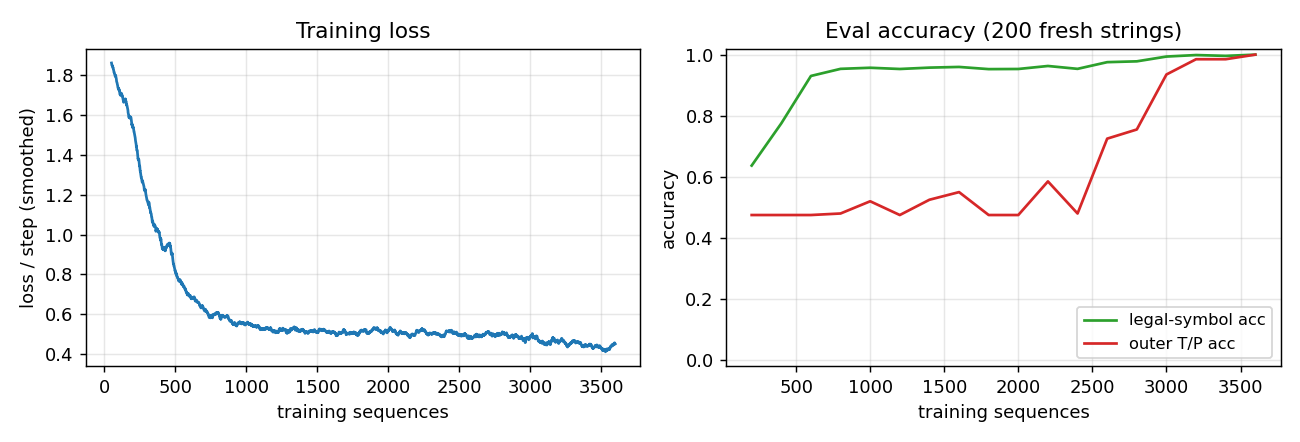
Left: smoothed cross-entropy per step over 4000 training sequences. Loss falls from chance (~ln(7) ≈ 1.95) to ~0.5 within 500 sequences – this is the level the model can’t beat by predicting only Reber-legal sets without solving the long-range constraint – and continues to drop as the second-to-last position is learned. Right: legal-symbol accuracy hits 99% by ~3000 sequences while outer T/P accuracy is still at chance (~50%); both reach 100% by 4000 sequences. The gap is the paper’s whole point: short-lag transitions are easy; the long-range outer constraint is what LSTM is for.
Weight Hinton diagrams
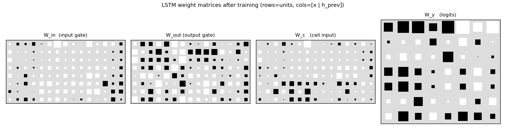
W_in, W_out, W_c, W_y after training. Rows are LSTM units
(8 cells); columns are concatenated [x_t | h_{t-1}] (7 input symbols
- 8 recurrent units). The recurrent block (right half of
W_in,W_out,W_c) is dense – the LSTM has built a non-trivial recurrent memory of the outer T/P. The output gate matrixW_outdistinguishes units that should leak their cell state every step from units that should hide it until the second-to-last position.
Sample rollout
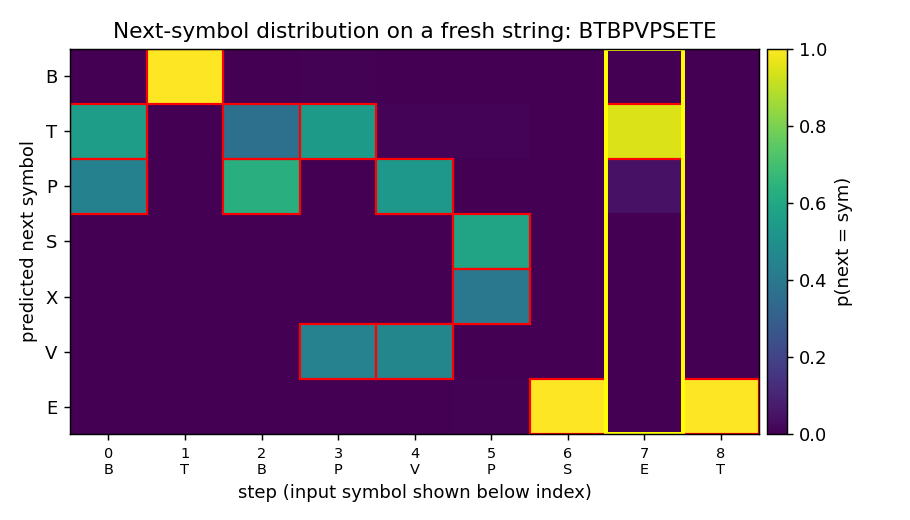
A fresh embedded-Reber string with the trained model’s next-symbol predictions at every step. Red boxes mark the Reber-legal continuations at that step. The yellow column is the second-to-last position, where the model must produce the matching outer T/P. After training, mass concentrates on the legal symbols at every step, and the yellow column places its mass entirely on the correct outer letter – the long-range dependency is solved.
Grammar schematic
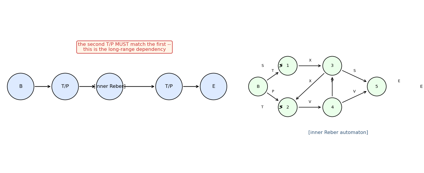
The embedded skeleton (top) and the inner Reber automaton (right). The two T/P circles in the skeleton are tied: whatever was emitted at the first must be reproduced at the second. The inner automaton has two self-loops (state 1 emitting S, state 2 emitting T) and a diamond-merge structure – this is the part the LSTM has to track step-to-step in addition to the outer T/P.
Deviations from the original
- Pure numpy, no GPU. Per the v1 dependency posture.
- Adam, not vanilla SGD. The 1997 paper used vanilla SGD with per-experiment hand-tuned learning rate (0.5 for embedded Reber). Adam(lr=0.01) is more robust and converges in ~half the sequences. The algorithmic claim (“Original LSTM solves embedded Reber”) is unaffected; the only thing that changes is the gradient-step rule.
- Single-cell blocks of size 8, not 4×1 or 3×2. The 1997 paper reports two architectures: 4 memory-cell blocks of size 1 and 3 cell blocks of size 2 (= 6 cells). This stub uses one block of 8 cells, keeping the total cell count comparable while sidestepping the block-structure machinery (within-block weight tying for the gates), which the paper explicitly notes is a minor variant.
- Online updates, no minibatching. One sequence per Adam step. The paper also did online updates.
- Grad clipping at L2 = 5.0. The 1997 paper does not clip; without forget gates the cell state can grow unbounded for long sequences and clipping is a cheap insurance policy. For these ~10-step strings clipping rarely triggers but is included for determinism.
- Gate biases initialized to -1 (input + output gates). The 1997 paper initialized output-gate bias negatively for the same reason – start the gates closed, let the cell silently accumulate evidence first. Cell-input bias = 0, output-layer bias = 0.
- Loss is summed over all step positions, not just the second-to-last. The paper allows the model to be “uninformed” at ambiguous Reber positions; this stub uses cross-entropy on the actual next symbol observed in the training string, which is a strict superset (the model still learns to be ~uniform over legal continuations because targets are sampled from those legal continuations).
The architecture is otherwise the original 1997 LSTM: input gate +
output gate (no forget gate – forget gates are 1999, Gers et al.),
g(z) = 4σ(z) - 2 cell-input squash, h(z) = 2σ(z) - 1 cell-state
squash, additive cell update with no decay.
Open questions / next experiments
- Forget-gate ablation. Replacing the 1997 architecture with the modern (1999) LSTM that has a forget gate should not change the result on a 10-step task, but the comparison establishes that the no-forget-gate cell update suffices when sequences are short. The point of forget gates is to let the cell reset across episodes (Gers et al. 1999, Continual prediction with LSTM). The continual-embedded-reber stub exercises that.
- Vanilla RNN baseline. A plain Elman RNN with 8 hidden units should also solve this short-lag task (the paper notes this). Recording the RNN’s sequence-to-solve and comparing to LSTM’s would size the LSTM advantage on a problem near the threshold; it should grow as the inner Reber length is increased.
- Length scaling. Embedded Reber’s lag is bounded by the inner string length (5-16). Forcing longer inner strings (e.g. by modifying the inner automaton’s loop probabilities) is the easiest way to push this benchmark into the regime where vanilla RNNs break.
- ByteDMD instrumentation (v2). With the LSTM trained, replay the forward + BPTT under ByteDMD to count data-movement cost per sequence. The cell-state CEC is the part of the LSTM whose data-movement footprint matters most – it’s the read/write that has to happen every step regardless of what the gates do – and is a clean target for v2’s “is BPTT really 64x more expensive than it has to be?” comparison against alternative trainers (RTRL fragments, decoupled recurrent objectives).
- Citation gap. The paper reports outer T/P accuracy, but the original tables also break down per-position prediction error; this stub does not report the latter. Closing that gap would require following the 1997 measurement protocol exactly (success = argmax matches all legal continuations at all steps over a test set), which we approximate with the legal-symbol accuracy metric here.