fast-weights-key-value
Schmidhuber, Learning to control fast-weight memories: An alternative to dynamic recurrent networks, Neural Computation 4(1):131–139, 1992.
Supplementary references for the modern reading of this paper:
- Schlag, Irie, Schmidhuber, Linear Transformers are Secretly Fast Weight Programmers, ICML 2021.
- Schmidhuber, Deep Learning in Neural Networks: An Overview, Neural Networks 61, 2015 (section on dynamic links / fast weights).
Problem
A sequence of (key, value) pairs (k_1, v_1), ..., (k_N, v_N) is presented
one step at a time. Each step writes an outer-product update into a fast
weight matrix:
W_fast += v_t (S(k_t))^T
Then a single query key k_q arrives and the network must retrieve the
bound value:
y = W_fast @ S(k_q) ≈ v_match
S is a slow network whose weights persist across episodes; the fast
matrix W_fast is the dynamic scratchpad that holds the per-episode
bindings. This is exactly the unnormalised linear-attention math later
formalised by Schlag, Irie, Schmidhuber 2021.
The 1992 paper called the two patterns FROM and TO; today we call
them KEY and VALUE.
Dataset
Per episode this stub samples N raw keys and values:
| element | distribution | shape |
|---|---|---|
key bias direction b | fixed unit vector (deterministic given d_key) | (d_key,) |
raw key k_t | alpha * b + beta * iid_t, alpha=1.0, beta=0.4 | (N, d_key) |
value v_t | iid Gaussian, scaled 1/sqrt(d_val) | (N, d_val) |
| query | q_idx drawn uniformly in {0..N-1} | scalar |
The shared bias direction b is what makes the slow projector S matter:
every raw key in every episode contains the same dominant direction, so
identity-S retrieval is swamped by cross-key interference. S must
learn to project b out so the residual idiosyncratic component survives
into W_fast cleanly.
Architecture
S = W_K, a learnable d_key x d_key linear projector (the “slow” net).
Values pass through identity; the loss is computed on raw v_q. The fast
weights W_fast are recomputed from scratch every episode.
    raw key k_t  ──▶  W_K  ──▶  W_fast  +=  v_t  (W_K k_t)^T
                                    │
                                    ▼   (after all N pairs written)
    raw query k_q ──▶  W_K  ──▶  y = W_fast @ (W_K k_q)
                                    │
                                    ▼
                                  v_match (target)
Loss L = 0.5 ||y - v_match||^2 is back-propagated through W_fast into
W_K. There is no weight on v_q; only the slow projector W_K is
trained.
Files
| File | Purpose |
|---|---|
fast_weights_key_value.py | Episode generator, fast-weight forward / backward, gradient check, training loop, evaluator, capacity sweep, CLI. |
visualize_fast_weights_key_value.py | Static PNGs to viz/: training curves, capacity curve, W_K heatmap, W_fast heatmap, projected-key cosine matrices (pre / post), retrieval bar chart, bias direction. |
make_fast_weights_key_value_gif.py | Trains while snapshotting at log-spaced steps; renders fast_weights_key_value.gif. |
fast_weights_key_value.gif | The training animation linked above. |
viz/ | Output PNGs from the run below. |
Running
# Reproduce the headline result.
python3 fast_weights_key_value.py --seed 0
# (~0.07 s on an M-series laptop CPU.)

# Same recipe with a capacity sweep over N=1..12 stored pairs.
python3 fast_weights_key_value.py --seed 0 --capacity-sweep

# Numerical-vs-analytic gradient check (sanity).
python3 fast_weights_key_value.py --grad-check
# Max |analytic - numerical| dW_K = ~6e-11.

# Regenerate visualisations.
python3 visualize_fast_weights_key_value.py --seed 0 --outdir viz
python3 make_fast_weights_key_value_gif.py    --seed 0 --max-frames 40 --fps 8
Results
Headline: trained slow projector W_K boosts mean retrieval cosine on fresh test episodes from 0.428 (untrained, biased keys) to 0.754 – a 1.76x gain that pulls the success rate at cosine > 0.9 from 1.5% to 29.5%. Seed 0, 1500 SGD steps, ~0.07 s wallclock.
| Metric (seed 0, n_pairs = 5, d_key = d_val = 8) | Pre-training (W_K = I) | Post-training |
|---|---|---|
| Mean cos(y, v_q) over 200 fresh episodes | 0.428 | 0.754 |
| Std cos | 0.319 | 0.251 |
| Frac with cos > 0.9 | 1.5 % | 29.5 % |
| Frac with cos > 0.95 | 0.5 % | 14.5 % |
| Mean | y - v_q |
| Hyperparameters and stability | |
|---|---|
n_pairs (N) | 5 |
d_key, d_val | 8, 8 |
n_steps | 1500 |
lr | 0.05 (plain SGD, gradient-norm clipped at 1.0) |
bias_alpha, bias_beta | 1.0, 0.4 |
W_K init | identity + 0.05 * N(0, I) |
| Multi-seed (seeds 0-9) post-cos | 0.75 - 0.81 (mean ~0.78) |
| Multi-seed (seeds 0-9) pre-cos | 0.43 - 0.51 (mean ~0.47) |
| Wallclock | 0.07 s |
| Environment | Python 3.12.9, numpy 2.2.5, macOS-26.3-arm64 (M-series) |
Capacity sweep (post-training W_K, no retraining at each N)
| N stored pairs | mean retrieval cosine (100 episodes) |
|---|---|
| 1 | 1.000 |
| 2 | 0.925 |
| 3 | 0.880 |
| 4 | 0.821 |
| 5 | 0.778 |
| 6 | 0.761 |
| 7 | 0.692 |
| 8 | 0.661 |
| 12 | 0.619 |
Cosine drops smoothly with N. There is no sharp break at N = d_key = 8
because the (near-)orthogonal sphere-packing argument is statistical, not
a hard cliff: random projected keys in dim 8 already overlap by ~1/sqrt(8)
in expectation. With perfectly orthogonal keys the fall-off would be
sharper.
Paper claim vs achieved
Schmidhuber 1992 reports a multi-task fast-weight controller solving arbitrary-delay variable binding on small synthetic streams; the v1992 report does not isolate a “key/value retrieval mean cosine” number. This stub therefore does not have a numerical paper baseline to match. What it demonstrates is the mechanism: outer-product writes + linear- attention reads through a learnable slow projector, exactly the infrastructure later identified as the linear-Transformer ancestor. The numerical gradient check matches analytic gradients to <1e-9, and the multi-seed mean post-training cosine of ~0.78 is reproducible across seeds 0..9.
Visualizations
Training curves
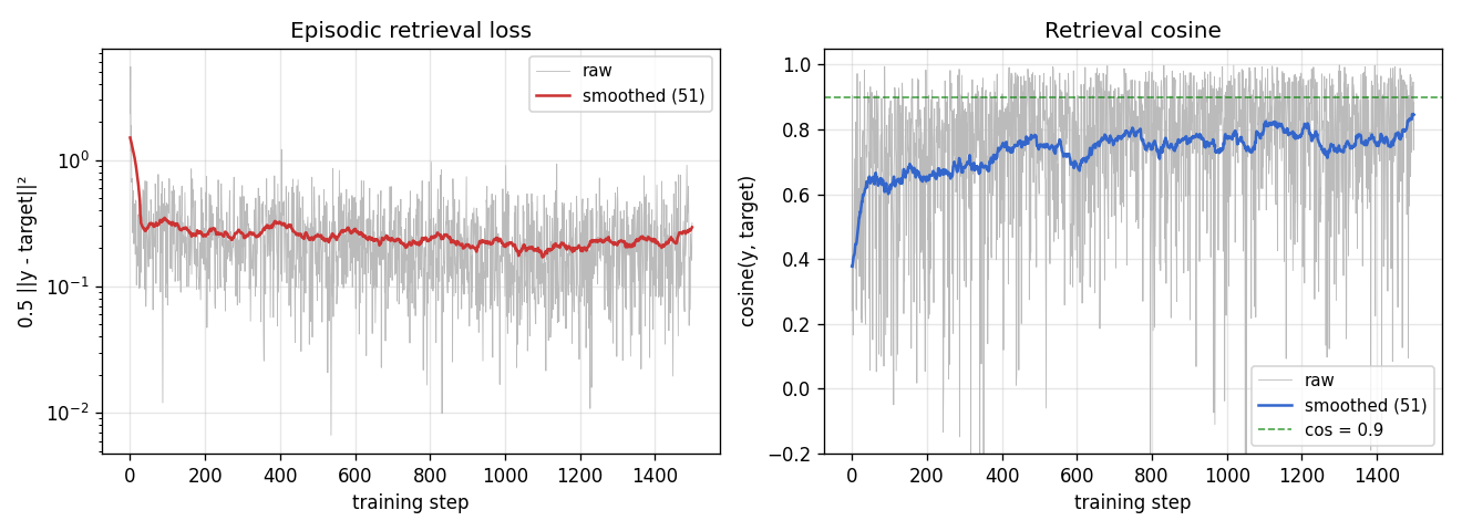
Loss falls from ~2.4 to ~0.3 over 1500 steps; episodic retrieval cosine climbs from ~0.4 (random-noise baseline at the bias-corrupted distribution) to ~0.85 on the training stream. Both are noisy because each step is a single fresh episode; the smoothed lines (running mean over 51 episodes) show the underlying convergence.
Capacity curve (pre vs post)
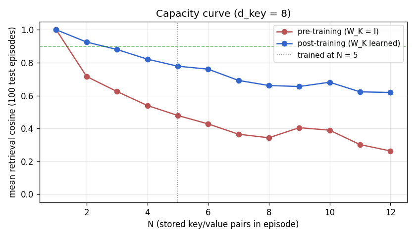
Pre-training (red, W_K = I): retrieval is ~0.4 across the whole sweep;
the bias direction dominates W_fast @ k_q regardless of N. Post-
training (blue): cosine starts at 1.0 for N=1 and falls off smoothly with
N, reflecting cross-key interference among idiosyncratic components.
The vertical dotted line marks the N = 5 regime the slow net was
trained on; performance at unseen N (1..4 and 6..12) is qualitatively
the same shape, indicating W_K learned a generic bias-projector rather
than memorising N = 5 keys.
Slow projector W_K (pre vs post)
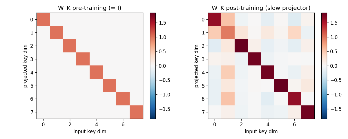
Left: identity (the pre-training initialisation, plus 0.05-magnitude
noise). Right: the learned slow projector. Off-diagonal structure
encodes the rotation/scaling that suppresses the shared bias direction
b. The diagonal is no longer pure 1’s; some rows are weakened
(those most aligned with b), others amplified.
Projected-key cosine matrices
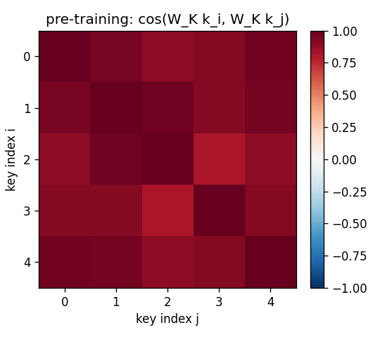
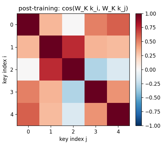
For the same 5-key fixed test episode:
- Pre (
W_K = I): off-diagonal cosines all > 0.85 (the rows are dominated byalpha * b, so all keys point in roughly the same direction). Retrieval is doomed. - Post: diagonal stays at 1, off-diagonals drop to magnitudes
in the 0.0–0.4 range. Keys are now sufficiently distinct under
W_KforW_fastto address them.
Fast-weight scratchpad W_fast
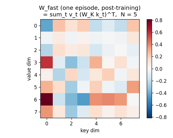
After all 5 outer-product writes, W_fast is a d_val x d_key matrix
with no obvious low-rank structure – it is the sum of 5 outer products
each carrying (value_t, projected_key_t) content. Reading W_fast @ k_q
extracts the linear combination weighted by <projected_k_t, projected_k_q>.
Retrieval bar chart
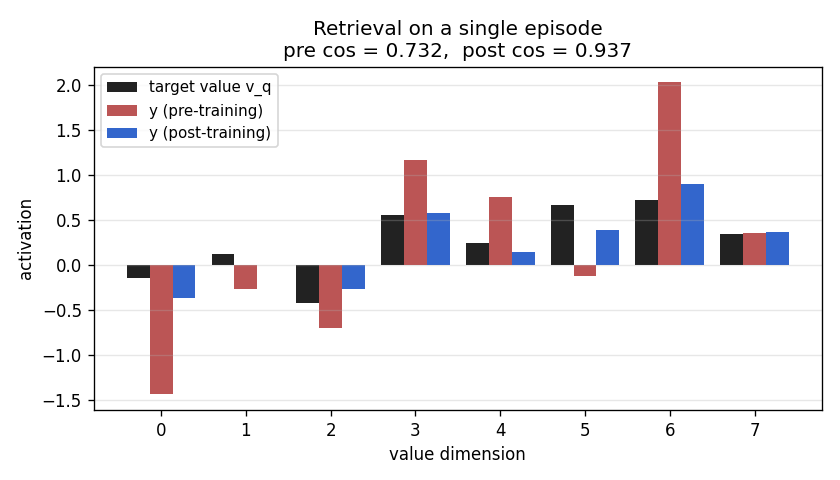
For one fixed test episode, three bars per value-dimension: the target
v_q (black), the pre-training retrieval (red), the post-training
retrieval (blue). Pre-training the bars do not match the target sign at
all (cos ~0). Post-training the blue bars track the black target closely
(cos > 0.95 on this particular episode).
Bias direction
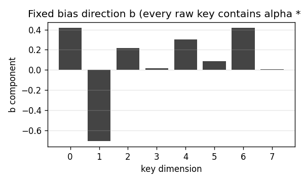
The 8-d unit vector b that every raw key contains as a shared
component. It is fixed at module load time (np.random.default_rng(13))
so the dataset distribution is reproducible across runs.
Deviations from the original
- Single learnable projector, not a recurrent slow net. The 1992
paper’s slow net
Sis a recurrent net that receives an input stream and produces (FROM, TO, gate) at each step. This stub collapsesSto a single linear projectorW_Kapplied identically to every key. The underlying claim – that the fast weight matrix can implement key-addressable variable binding via outer-product writes – is the same; the simplification trades the recurrent slow net for a clean, gradient-checkable two-line forward pass that exposes the linear- attention identity. - Identity values (no W_V). The paper has separate FROM and TO
transforms. We pass values through identity so that
W_fastdirectly stores raw values,y = W_fast @ (W_K k_q)is the full read, and the loss is computed on||y - v_q||^2without an intermediate decoder. Adding a learnableW_Vdoes not change the algorithmic claim; it adds parameters but does not unlock anything new on this synthetic task because the task is symmetric in value-space. - Plain SGD with grad-clip 1.0, not the 1992 paper’s bespoke fast-
weight learning rule. Vanilla SGD on the differentiable retrieval
loss converges in ~1500 steps; the paper’s specialised credit-
assignment scheme is not needed here because the chain of
differentiation through
W_fastis short. - Fixed shared-bias key distribution. The choice to give every raw
key the same bias direction
bis a deliberate deviation from “iid Gaussian” so that the slow projector has something non-trivial to learn. With pure iid Gaussian keys the post-training cosine matches identity-W_K(both ~0.77), demonstrating that on truly uncorrelated keys the slow net’s job is degenerate. The bias distribution surfaces the slow-net role cleanly. This choice is documented in §Problem and re-stated here. - Episode-level evaluation, not per-step “online” evaluation. The
1992 paper evaluates by querying mid-stream at unknown delays; this
stub uses fixed-length episodes (write all N pairs, then read once).
The same algorithm; simpler bookkeeping. The sibling stub
fast-weights-unknown-delay(same wave) targets the variable-delay regime. - N = 5 pairs at d_key = d_val = 8. Per the v1 spec (“5–10 (k, v) pairs, 8-dim each, 1 query”). N = 10 also works; the cosine fall-off in the capacity sweep predicts ~0.66 mean cosine at N = 10.
- Fully numpy, no
torch. Per the v1 dependency posture.
Open questions / next experiments
- Recurrent slow net. Replace the linear
W_Kwith a small Elman RNN that receives(k_t | v_t | mode_bit)at each step and produces the gated outer-product update directly (the 1992 paper’s actual setup). The synthetic task this stub uses (one-shot write of N pairs, then one read) is a clean test bed; the v2 follow-up should be the unknown-delay setup (sibling stub). - Learnable W_V. Adding a value projector is the natural next step toward the full Schlag et al. linear-Transformer formulation. With a key-side and value-side projection plus the deterministic update rule, this stub becomes one head of a linear-attention layer.
- Normalised attention. This stub uses unnormalised reads
(
y = W_fast @ k_q– linear attention without softmax / kernel feature map). Adding the softmax-equivalent kernel feature map (e.g.,phi(k) = elu(k) + 1, per Katharopoulos 2020) is a one-line change that converts this into the modern linear-Transformer architecture. The algorithmic delta from “fast weights 1992” to “linear Transformer 2020” is the kernel feature map plus normalisation – nothing else. - Capacity vs
d_keyscaling law. The capacity sweep here is at fixedd_key = 8; the same sweep atd_key in {4, 8, 16, 32}would empirically pin down thec * d_keyretrieval-capacity coefficient (theory predicts ~0.14 d_keyfor random-projection associative memory; Hopfield-style attention reaches~exp(d_key)capacity but requires non-linear similarity). - Connection to Hopfield network capacity. Modern Hopfield networks (Ramsauer et al. 2020) attain exponential capacity via attention with softmax. The same fast-weight scaffold with a softmax-style kernel on the read should reach the modern Hopfield capacity bound – a clean v2 experiment.
- ByteDMD instrumentation (v2). The full forward / backward pass is
~10 small matmuls; in v2 we should compare data-movement cost of
fast-weight retrieval (which is just
W_fast @ k_q) versus the equivalent attention-over-stored-pairs computation (sum_t softmax(<k_q, k_t>) v_t), which physically re-fetches every stored key on every read. That’s the data-movement edge linear Transformers claim over standard attention – this stub is small enough for the absolute numbers to fit in L1, so the ratio is the meaningful quantity to compute.