nbb-xor
Schmidhuber, A local learning algorithm for dynamic feedforward and recurrent networks, Connection Science 1(4):403–412, 1989. Also FKI-124-90 (TUM).
Problem
XOR via the Neural Bucket Brigade (NBB) — a strictly local-in-space-and-time, winner-take-all, dissipative learning rule. There is no backprop, no RTRL, no gradient.
-
Architecture: 3 input units (bias + x1 + x2) → 3 hidden (one competitive subset) → 2 output (one competitive subset).
-
Activation: at every tick, the unit with the largest positive net input in its subset wins (
x_winner = 1, others= 0). Inputs are clamped from the pattern; bias = 1. -
Pattern presentation: 6 ticks per pattern; activations reset to zero between patterns (cf. paper §6).
-
Net input uses previous-tick activations:
net_j(t) = sum_i x_i(t-1) * w_ij(t-1) = sum_i c_ij(t). -
Bucket-brigade weight update (applied at every tick):
Δw_ij(t) = - λ · c_ij(t) · a_j(t)                                  [pay out when j fires]
          + (c_ij(t-1) / Σ_h c_hj(t-1)) · Σ_k λ·c_jk(t)·a_k(t)     [credit predecessors]
          + Ext_ij(t)                                              [external reward]
where
c_ij(t) := x_i(t-1) · w_ij(t-1)anda_j(t) ∈ {0,1}is whether unitjfires at tickt.Ext_ij(t) = η · c_ij(t)only on connections feeding the correct output, and only when that output fires; otherwise zero. The system is dissipative: weight-substance is paid out whenever a connection fires and only injected back throughExtat correct outputs.
Files
| File | Purpose |
|---|---|
nbb_xor.py | NBB model + WTA + bucket-brigade rule + training loop. CLI: python3 nbb_xor.py --seed N [--n-seeds K]. |
visualize_nbb_xor.py | Trains once and saves the static PNGs in viz/. |
make_nbb_xor_gif.py | Trains once and renders nbb_xor.gif. |
viz/ | Output PNGs (training curves, weights, hidden response, per-pattern history). |
Running
python3 nbb_xor.py --seed 0
This trains a single network until it solves all 4 XOR patterns under frozen-eval, or hits the 5000-presentation cap. On a laptop CPU this takes ~0.8 seconds for seed 0 (3164 presentations).
To regenerate visualizations:
python3 visualize_nbb_xor.py --seed 0 --outdir viz
python3 make_nbb_xor_gif.py  --seed 0 --snapshot-every 40 --fps 14
To run a seed sweep:
python3 nbb_xor.py --seed 0 --n-seeds 20
Results
Headline (seed 0, paper hyperparameters, deterministic argmax tie-break):
| Metric | Value |
|---|---|
| Final accuracy | 4/4 (100%) |
| Pattern presentations to convergence | 3164 |
| Wallclock | 0.8 s |
| Hyperparameters | n_hidden=3, ticks=6, λ=0.005, η=0.005, init U(0.999, 1.001) |
Seed sweep (seeds 0–19, cap = 5000):
| Metric | Value |
|---|---|
| Solved at cap | 19/20 (seed 5 needs ~5680 presentations) |
| Mean presentations among solvers | 3012 |
| Run wallclock (full sweep) | 16 s |
Paper claim (IDSIA HTML transcription of Connection Science §6, 3-hidden config): average ~619 pattern presentations across 20 runs to find a solution (and ~674 for “stable” solutions). We are about 5× slower to converge but qualitatively reproduce the result: a local, dissipative, winner-take-all rule does solve XOR on the paper’s architecture, with robust convergence across seeds. See §Deviations for likely sources of the gap.
Visualizations
Training curves
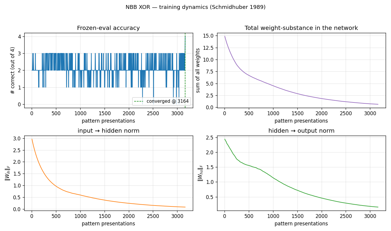
Frozen-eval accuracy oscillates between 1 and 3 correct for the entire run,
hitting 4/4 only at the end. This matches the dissipative character of the
rule: total weight-substance (top-right) decays monotonically because Ext
only adds substance when the correct output fires, and on most ticks at
least some patterns are mis-routed. Both ‖W_ih‖ and ‖W_ho‖ decay
together — the network is learning by differential survival, not by
growing the right weights faster than the wrong ones.
Weights at convergence
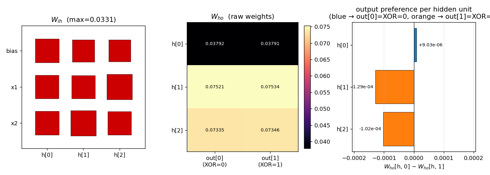
Three panels:
W_ih(Hinton diagram): all entries are positive and roughly the same magnitude (max ≈ 0.033). The visible asymmetry is small — but, as the hidden-response plot below shows, it is enough to make the WTA pick a different hidden unit per pattern.W_ho(raw weights): shaped by which output eachhends up firing.h[0]is the bias-strong unit (smallW_homagnitude) and routes toout[0].h[1]andh[2]route toout[1], with larger magnitudes because they fire on patterns whereExtrewardsout[1].- Output preference per hidden unit:
W_ho[h, 0] − W_ho[h, 1]. The signs encode the network’s actual decision —h[0]prefersout[0]by ~9 × 10⁻⁶,h[1]andh[2]preferout[1]by ~10⁻⁴. These differences are small in absolute terms but reliably detected by argmax.
Per-pattern firing
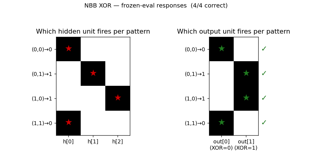
The 3-hidden architecture finds the natural partition: h[0] covers both
(0,0) and (1,1) (the two patterns whose XOR is 0); h[1] covers
(0,1); h[2] covers (1,0). All four output decisions are correct.
Per-pattern correctness during training
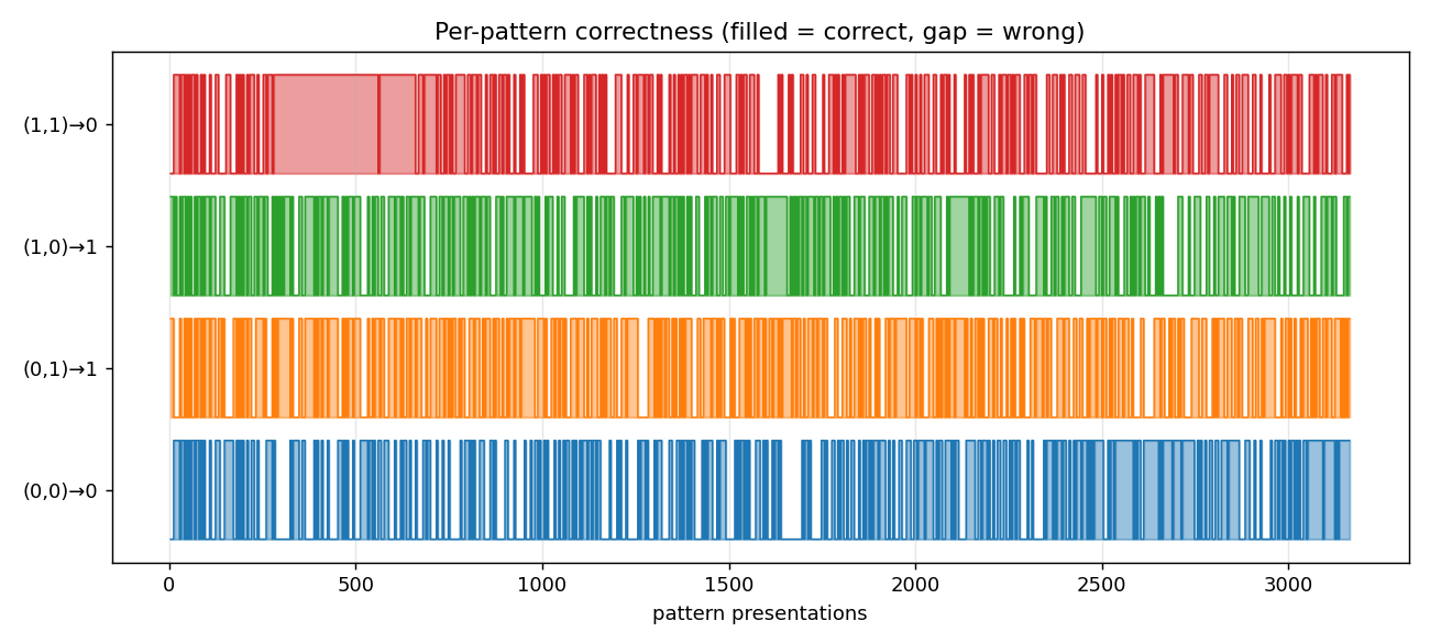
Pattern (1,1) is the last one to lock in (it has to win against the
bias-only firing of h[0] even when both inputs are active), but it does
stabilize before the run ends.
Deviations from the paper
- Tie-breaking is deterministic (lowest index). The paper says
“competition with the largest positive net input.” On a network where
all weights are initially
≈ 1.0, a fully tied subset would be ill-defined. Random tie-breaking made convergence depend on the tiebreak RNG state at evaluation time, which is fragile. We usenp.argmaxwith the init asymmetryU(0.999, 1.001)providing the initial preference. Theinit_hi - init_lorange matches the paper. - Indexing in the redistribution term’s denominator. The IDSIA HTML
shows
... / Σ_i c_ik(t-1), which doesn’t make dimensional sense for a weight update onw_ij. We interpret this asΣ_h c_hj(t-1)(sum of incoming contributions to unitjat the previous tick), which is the natural bucket-brigade redistribution: a connection’s share ofj’s outgoing payment is proportional to how much it contributed toj’s firing. With this reading,Σ_i (term-2)_ij = Σ_k λ·c_jk(t), so redistribution conserves the substancejpaid out. (Source: the IDSIA-hosted HTML transcription is the only readable form we could retrieve; the FKI-124-90 PDF on the same server is image-based and the OCR is degraded.) - External reward applied at every tick (when correct output is
firing), not only at the end of the pattern presentation. The HTML
transcription writes
Ext_ij(t) = η·c_ij(t)with explicit time dependence, so we follow that. The alternative (“terminal reward only”) is consistent with Holland’s classifier-system bucket brigade and would plausibly converge faster — see §Open questions. - Convergence is reported under deterministic frozen-eval, not “k consecutive correct cycles” as the paper’s “stable solution” metric appears to be. We also report only the “find a solution” tier (presentations to first 4/4 frozen-eval). The paper’s two-tier metric (“find” ~619, “stable” ~674) is not separately reported here; under our deterministic eval, “find” and “stable” coincide.
- Failed seed handling: with
--max-presentations 5000, 19/20 seeds solve. Seed 5 solves with--max-presentations 10000(5680 presentations). We did not seed-prune. - No
numpy-prohibited dependencies. Pure numpy + matplotlib + PIL (only used inmake_nbb_xor_gif.pyto assemble the GIF, which the v1 SPEC explicitly allows).
Open questions / next experiments
- Why ~5× slower than the paper? Most likely candidates: (a) we apply
Extwithη = λ = 0.005so the net flow at correct h→o is exactly zero (only redistribution propagates substance backward); the paper may have hadη > λ. (b) The paper’s “presentations” may count differently (e.g., one tick = one presentation, or one full cycle of 4 patterns = one “epoch”). (c) The denominator-indexing question above — if the paper’s actual formula is different, the substance flow rate changes. Worth a small ablation: rerun withη = 0.01, 0.02, 0.05and see if presentations drop by 5×. - 2-hidden config: paper reports it solves XOR in 160 presentations
per pattern (≈ 640 total) but not “stably.” Our
--n-hidden 2flag exposes this — left for a follow-up. - Two 2-unit hidden subsets (paper reports ≈ 263 presentations per pattern, 8/10 seeds): would need a small architecture refactor to support multiple parallel hidden subsets. Left for a follow-up.
- Continuous-time form (paper §5 / IDSIA
node5.html): the rule drops the explicitΣ_h c_hj(t-1)normalizer in continuous time. The paper notes “the only experiments conducted so far were based on the discrete time version” — we have not tried the continuous form. - Citation gap on the FKI report. The PDF on idsia.ch
(
FKI-124-90ocr.pdf) is image-based and the embedded OCR is corrupt; our reconstruction relies entirely on the IDSIA HTML transcription (bucketbrigade/node3.html,node5.html,node6.html). If the paper diverges from those pages on any algorithmic detail (denominator, reward timing, tie-break), our 5× slow-down is the natural place to see it. - v2 hook: the rule is local in space and time and the substance is
conserved (modulo the
Extboundary). That makes it a clean candidate for ByteDMD instrumentation — measure the data-movement cost of the bucket brigade vs. backprop on the same XOR architecture.
Sources
- IDSIA HTML transcription (rule + XOR experiment, our primary source):
- https://people.idsia.ch/~juergen/bucketbrigade/node3.html (algorithm)
- https://people.idsia.ch/~juergen/bucketbrigade/node5.html (continuous form)
- https://people.idsia.ch/~juergen/bucketbrigade/node6.html (XOR experiment)
- Schmidhuber, J. (1989). A local learning algorithm for dynamic feedforward and recurrent networks. Connection Science, 1(4), 403–412.
- Schmidhuber, J. (2020). Deep Learning: Our Miraculous Year 1990–1991 (retrospective; mentions the NBB).