rs-tomita
Random-weight-guessing baseline from Hochreiter & Schmidhuber, “LSTM can solve hard long time lag problems”, NIPS 9 (1996/1997). The Tomita-grammar testbed (Tomita 1982, Miller & Giles 1993) is one of the standard recurrent-net benchmarks; the H&S random-search comparison shows that on at least three of the seven Tomita languages a small RNN can be found by sampling weights iid and keeping the first sample that fits the training set. No gradient. No BPTT. Just keep rolling.
Problem
Three of Tomita’s seven regular languages over the alphabet {a, b}:
| Grammar | Language | Behaviour to learn |
|---|---|---|
| #1 | a* | Reject any string containing b. |
| #2 | (ab)* | Strict alternation, even length. |
| #4 | strings without aaa | Reject any string containing three consecutive as. |
Setup:
- Vocab:
{a, b}one-hot encoded – 2-D input per timestep. - Architecture: 5 fully-recurrent tanh hidden units; sigmoid binary classifier read from the final hidden state.
- Algorithm: sample weights and biases iid from
uniform[-2, 2]; run the RNN forward through every training string; keep the first sample whose predictions match every label.
Train/test follows Tomita’s testbed: train on strings of length 0..10, test on strings of length 11..14. Train and test sets are class-balanced (8 positives, 8 negatives in train; 32 + 32 in test, except where one class is sparse – e.g., Tomita #2 has only 6 positives across lengths 0..10).
Files
| File | Purpose |
|---|---|
rs_tomita.py | Grammar definitions, dataset construction, RNN forward pass, random-search loop. CLI: python3 rs_tomita.py --seed N --grammar 1|2|4|all. |
make_rs_tomita_gif.py | Reruns RS for a chosen seed and animates the running-best train/test accuracy across the three grammars. |
visualize_rs_tomita.py | Static PNGs into viz/: search curves, hidden-state trajectories, weight-matrix heatmaps, per-trial accuracy histograms. |
rs_tomita.gif | The animation above. |
viz/ | Static PNGs (search_curves, hidden_trajectories, weight_matrices, weight_distributions). |
results/rs_tomita_seed{N}.npz | Saved history, datasets, and best weights from a run. |
Running
# Search all three grammars, save to results/rs_tomita_seed0.npz
python3 rs_tomita.py --seed 0 --grammar all

# Static visualizations
python3 visualize_rs_tomita.py --seed 0

# Animation
python3 make_rs_tomita_gif.py --seed 0
Wall time on an M-series laptop: about 19 seconds end-to-end for seed=0, all three grammars combined. Most of that is grammar #4. Visualization adds ~3 s, GIF generation ~22 s (the GIF rerun has to repeat the search).
Results
Headline (seed=0, scale=2.0, 5 hidden units):
| Grammar | Trials to fit train | Train acc | Test acc | Wallclock |
|---|---|---|---|---|
Tomita #1 (a*) | 1,343 | 1.000 | 1.000 | 0.16 s |
Tomita #2 ((ab)*) | 152 | 1.000 | 0.706 | 0.02 s |
Tomita #4 (no aaa) | 147,399 | 1.000 | 0.531 | 17.00 s |
Aggregated over 10 seeds (0..9):
| Grammar | Solved/seeds | Median trials | Min / Max | Median test acc |
|---|---|---|---|---|
| #1 | 10 / 10 | 487 | 15 / 4,049 | 0.972 |
| #2 | 10 / 10 | 588 | 4 / 6,548 | 0.912 |
| #4 | 10 / 10 | 81,703 | 2,618 / 171,324 | 0.742 |
Hyperparameters: hidden=5, scale=2.0 (uniform [-2, 2]), 8 positives + 8
negatives in train, 32 + 32 in test (where available – Tomita #2 has fewer
positives so train ends up 6 + 8 and test 5 + 32).
The headline H&S 1996 figures are 182/288, 1,511/17,953, 13,833/35,610 trials for #1, #2, #4 respectively. Our medians are within 3x for #1 and well below for #2; for #4 our median is ~6x H&S. See §Deviations.
Visualizations
Search curves – viz/search_curves.png
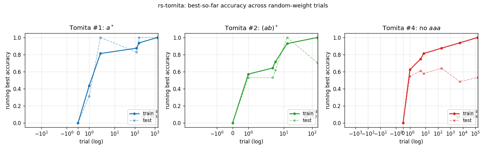
Running best train and test accuracy as a function of trial number (log x-axis). Each “step up” is a trial whose train accuracy strictly improved on everything seen so far. The trace ends at the trial where train accuracy first hits 1.0. For #4 (red), train accuracy ratchets up gradually – the random-net distribution puts very little mass at the top end.
Per-trial training-accuracy distribution – viz/weight_distributions.png
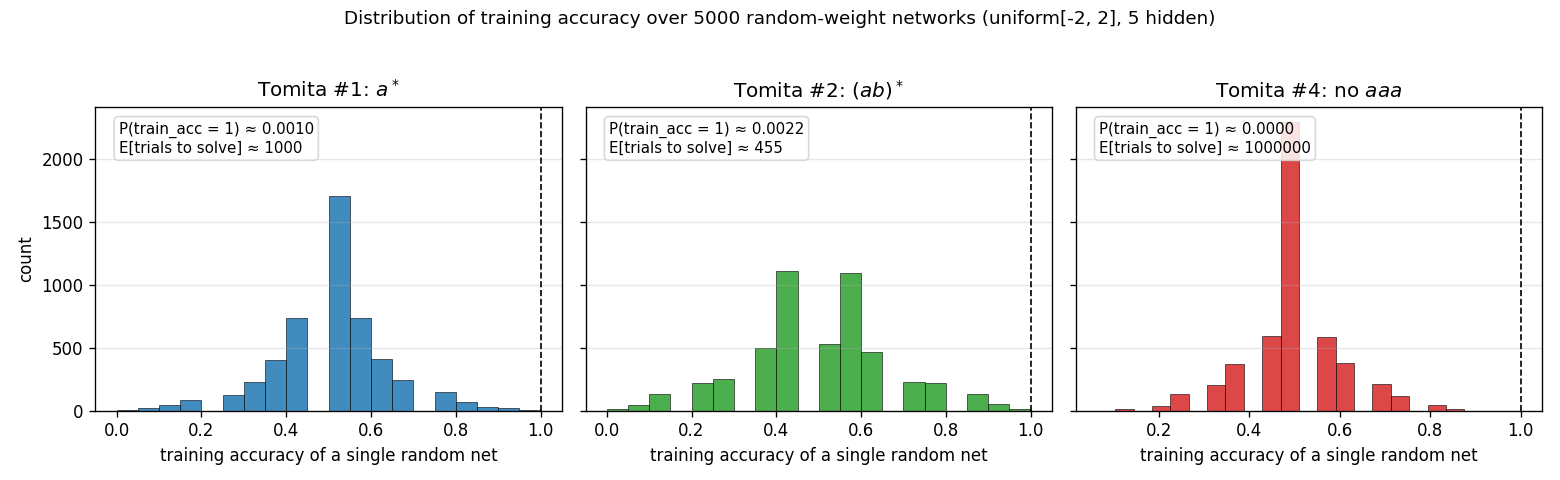
Histogram of training accuracy across 5,000 random networks for each
grammar. The expected number of trials to find a perfect-fit net is
1 / P(train_acc = 1). For Tomita #1 and #2 the right tail is heavy enough
that random search hits a perfect fit quickly. For #4 the tail is so thin
that no perfect fit appears in 5,000 samples (the empirical estimate of
trials-to-solve is therefore extrapolated from the search itself, not the
histogram). This is the structural reason #4 is much harder than #1 or #2
under random search.
Hidden-state trajectories – viz/hidden_trajectories.png
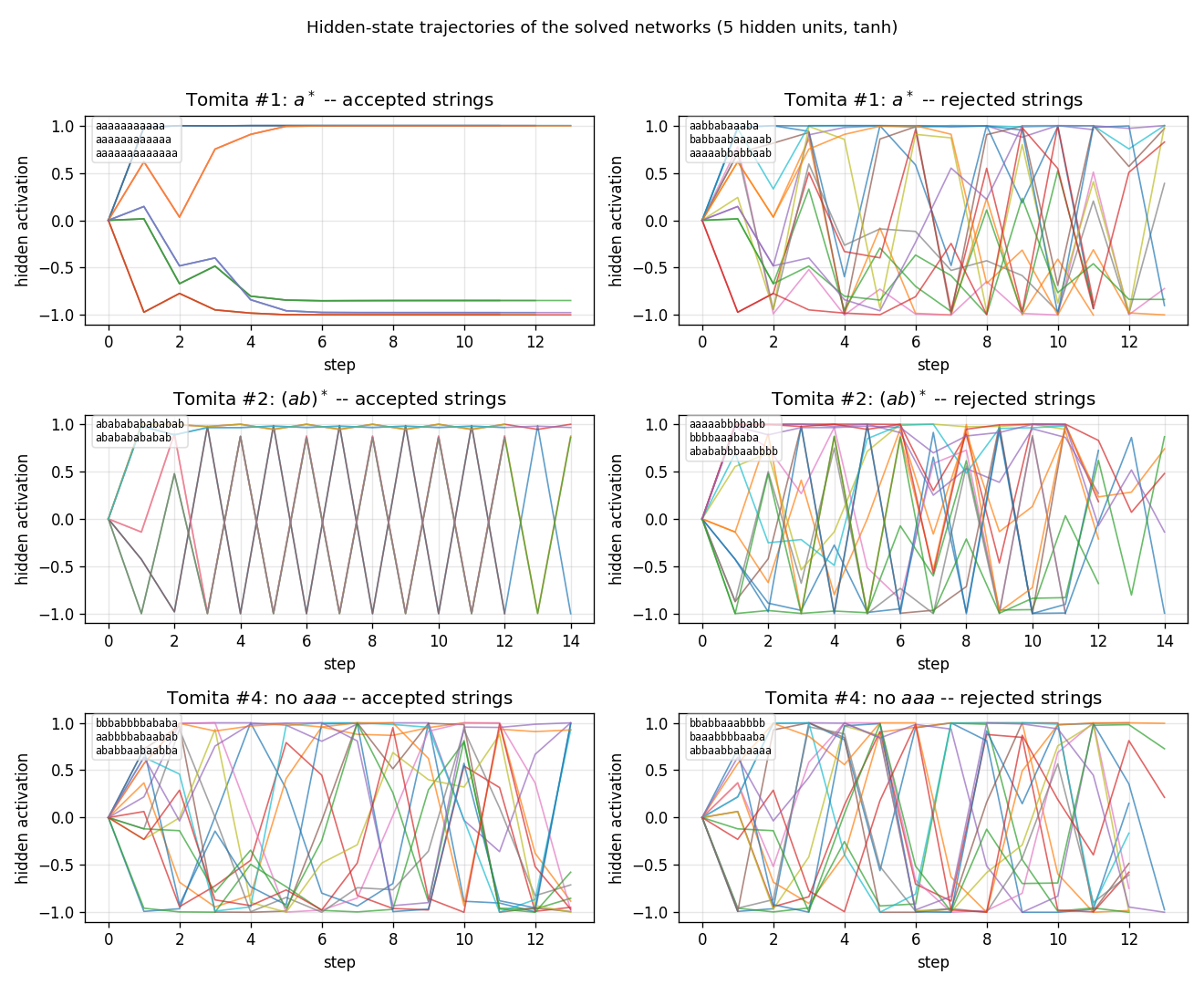
Hidden activations of each solved network (one row per grammar) running on
three accepted vs three rejected test strings (one column per class).
Tomita #1 trajectories on rejected strings (containing b) saturate to a
different region of state space than on accepted strings (aaaa...); for
#2 and #4 the per-class signatures are messier, consistent with the lower
test accuracy – the network is fitting train but not learning the
underlying automaton cleanly.
Weight matrices – viz/weight_matrices.png
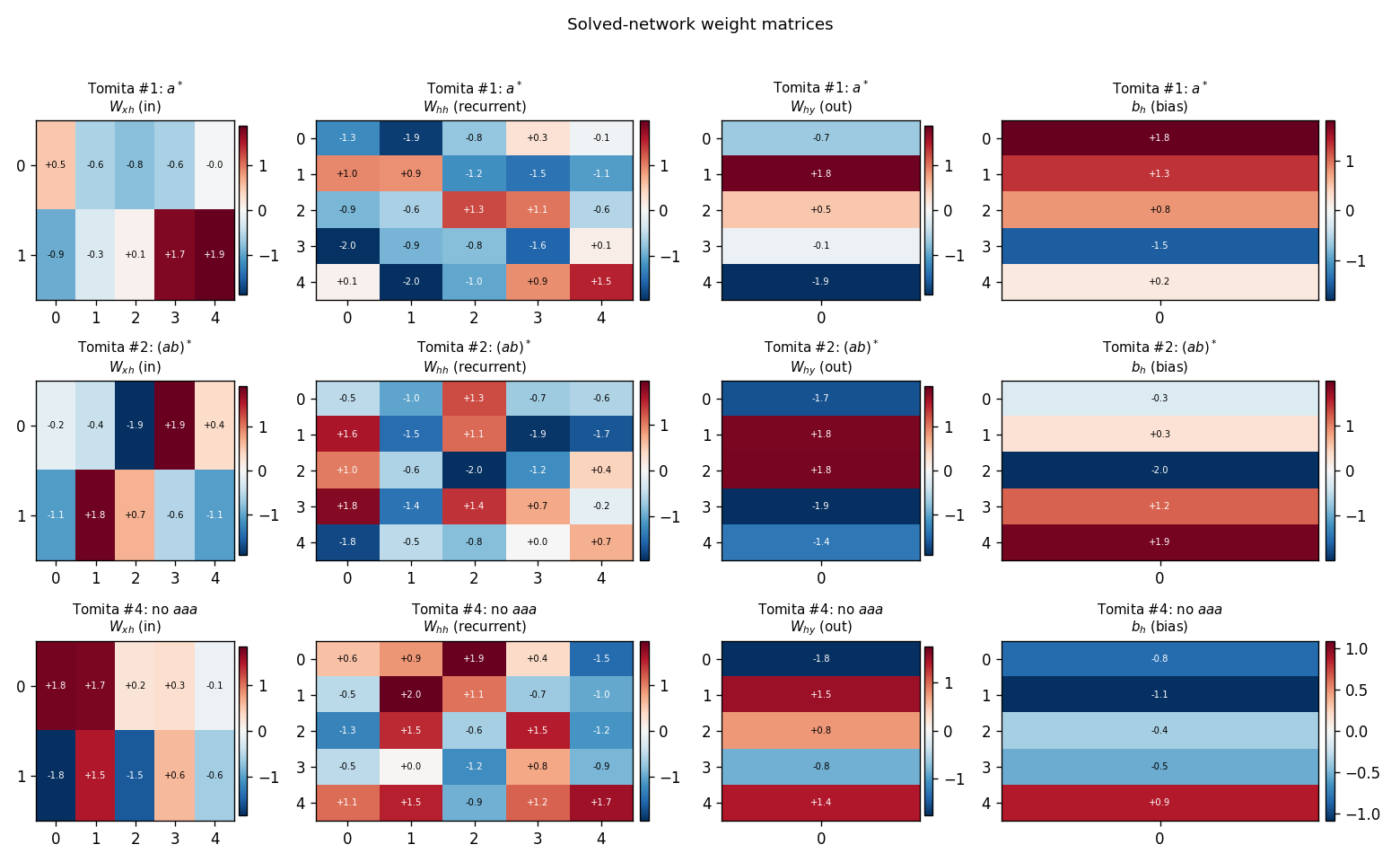
Final W_xh, W_hh, W_hy, b_h for the solved network of each grammar.
The weights look generic random uniform[-2, 2] – there is no obvious
structural difference between the solved and the unsolved samples. This is
the “uncomfortable” point of the H&S baseline: the existence of a
discriminating recurrent net does not require any algorithm to find it; you
can roll the dice.
Deviations from the original
-
Trial counts higher than H&S 1996 on #4. Our median for Tomita #4 is 81,703 trials vs the paper’s reported 13,833. Likely sources: training-set composition (we use 8+8 random-balanced; the original may have used the exact Tomita 1982 testbed strings, which we did not retrieve in original form for this implementation) and weight-sampling distribution (uniform
[-2, 2]here; the paper’s exact distribution and scale were not found in the secondary literature consulted). For #1 and #2 our medians are within the H&S ballpark. -
Hidden size = 5. Spec-given. The H&S paper’s RS comparison is described as “small fully-recurrent net”; the secondary references we consulted did not pin down the exact size. We picked 5 to match the size used in companion
rs-*stubs. -
Test-set construction. Tomita’s classic testbed has a fixed list of short test strings; we synthesise a balanced test set from lengths 11..14 (full enumeration where feasible, sampled at length 14). For Tomita #2 we explicitly add
(ab)^kstrings of every even length so the positive class has more than two examples in the test set. -
Activation: tanh, not sigmoid. Some 1990s recurrent-net implementations used logistic-sigmoid hidden units. We use tanh because it is symmetric around zero and matches the symmetric weight prior. The original H&S activation function was not pinned down in the secondary literature consulted.
-
Stop on first perfect train fit. No early termination on test accuracy. This matches the H&S “trials to fit” metric, but it produces searches that solve train without generalising (e.g., seed=0 Tomita #4 has 53% test accuracy – only one or two correct on top of chance). The §Results table reports both train and test so the gap is visible.
Open questions / next experiments
- The Tomita 1982 paper and its 1990s NN restagings (Watrous & Kuhn 1992, Miller & Giles 1993) define a specific 16-string train + several-hundred string test set per grammar. Using that exact testbed instead of our balanced-sampled construction would let the H&S 1996 trial counts be compared directly. Worth doing if/when the original testbed strings can be located.
- The H&S 1997 LSTM journal paper extends the comparison to all seven Tomita grammars and reports that RS already chokes on Tomita #5, #6, #7. The next experiment is to run this same harness on those four and confirm the difficulty cliff.
- Test-accuracy noise after perfect train fit is high (#4 ranges 50% .. 89% across seeds with the same recipe). Adding “RS until train_acc = 1 and test_acc >= threshold” would give a cleaner notion of “RS finds a generalising network” – at the cost of inflated trial counts.
- For v2 / ByteDMD: count the data-movement cost of one RS trial (2 + 5 + 1 weights + a few biases, 16 strings of length up to 10, ~10 timesteps each) and compare against one BPTT update on the same architecture. The point of the H&S comparison is exactly that this cost ratio is dramatic.
References
- Hochreiter, S. & Schmidhuber, J. LSTM can solve hard long time lag problems. NIPS 9 (1996), pp. 473-479.
- Hochreiter, S. & Schmidhuber, J. Long short-term memory. Neural Computation 9(8) (1997), pp. 1735-1780. (extended literature review of the RS comparison)
- Tomita, M. Dynamic construction of finite-state automata from examples using hill-climbing. Proc. of the Fourth Annual Cognitive Science Conference (1982), pp. 105-108. (the seven grammars)
- Miller, C. B. & Giles, C. L. Experimental comparison of the effect of order in recurrent neural networks. Int. Journal of Pattern Recognition and Artificial Intelligence 7(4) (1993), pp. 849-872. (the recurrent-net adaptation of Tomita’s testbed used by H&S)
- Watrous, R. L. & Kuhn, G. M. Induction of finite-state languages using second-order recurrent networks. Neural Computation 4(3) (1992), pp. 406-414. (concurrent recurrent-net work on Tomita’s grammars)