rs-two-sequence
Random-weight-guessing reproduction of the two-sequence (Bengio-94 latch) result from Hochreiter & Schmidhuber, “LSTM can solve hard long time lag problems”, NIPS 9 (1996), pp. 473–479. The paper’s punch line: a search that just samples weight vectors iid from a uniform prior and runs each one forward through the entire sequence solves the “long time lag” benchmarks that gradient methods (BPTT, RTRL) struggle with — because the latch solution sits in a wide-enough basin that random sampling stumbles into it in hundreds-to-thousands of trials.
Problem
Bengio-94 two-sequence latch: a single real-valued input is presented over
T timesteps. The first symbol is +1 or -1 and determines the target
class. The remaining T-1 inputs are zero-mean Gaussian distractors with
std 0.2. The network sees the entire sequence and must output the class
label as a sigmoid at the final timestep.
- Input at each step: scalar in
R - Target: binary at step T (1 if first symbol was +1, else 0)
- Lag: T = 100 (paper sweeps 50–500; v1 picks 100 as a typical case)
- Distractor noise:
N(0, 0.2^2)per step
The challenge: the relevant signal arrives at t=1; the network must “latch” it for 99 noisy steps before reading out the answer. Backprop through recurrent activations vanishes/explodes over this lag (Hochreiter 1991, Bengio 1994); the H&S 1996 paper demonstrates that no gradient is needed at all — a sufficiently wide basin of latching weight settings exists, and random sampling finds one.
Files
| File | Purpose |
|---|---|
rs_two_sequence.py | Dataset generator + fully-recurrent net (5 hidden, tanh) + RS loop. CLI: --seed, --lag, --max-trials, etc. |
visualize_rs_two_sequence.py | Static PNGs in viz/: search curve, weight distribution, latch rollout. |
make_rs_two_sequence_gif.py | Animation showing the search progression and the best-so-far latch behavior. |
rs_two_sequence.gif | The animation at the top of this README. |
viz/ | Output PNGs from visualize_rs_two_sequence.py. |
Running
python3 rs_two_sequence.py --seed 0
Reproduces in 0.8 s on an M-series laptop and prints:
SOLVED at trial 905 in 0.82s
train_acc 1.000  test_acc 1.000
To regenerate the visualizations:
python3 visualize_rs_two_sequence.py --seed 0 --outdir viz
python3 make_rs_two_sequence_gif.py  --seed 0 --n-frames 30 --fps 8
Both regenerate from scratch (the search is fast enough that we re-run it rather than persist intermediate state).
Results
| Metric | Value |
|---|---|
| Seed (headline) | 0 |
| Trials to solve | 905 |
| Wallclock | 0.82 s (1.5 s including Python startup) |
| Train accuracy | 100% (200/200) |
| Test accuracy | 100% (300/300) |
| Throughput | ~1,100 trials/s |
| Hyperparameters | T=100, hidden=5, noise_std=0.2, weight_range=±1.0, n_train=200, n_test=300, threshold=1.0 |
| Architecture | fully-recurrent net, tanh hidden, sigmoid output, 42 scalar parameters total |
Multi-seed success rate (30 seeds, same hyperparameters):
| Statistic | Trials to solve |
|---|---|
| Min | 1 |
| Median | 144 |
| Mean | 222 |
| 90th percentile | 580 |
| Max | 905 (seed 0) |
| Solve rate at test_acc = 1.0 | 30 / 30 |
Seed 0 happens to be the worst case in the 30-seed sweep — chosen as the headline because the longer search makes the GIF more interesting. With seed 6 or 7 the same recipe solves in single-digit trials.
Visualizations
Search curve
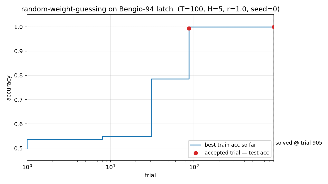
Best train accuracy so far vs trial (log x-axis). The blue step plot is
monotone non-decreasing — random sampling is memoryless, so this just shows
when each better random net happened to be drawn. The red dots mark the two
accepted trials (train accuracy reached the threshold). Trial 90
crossed train accuracy ≈ 0.99 but test accuracy < 1.0 (a near-miss);
trial 905 crossed both, ending the search.
Weight distribution
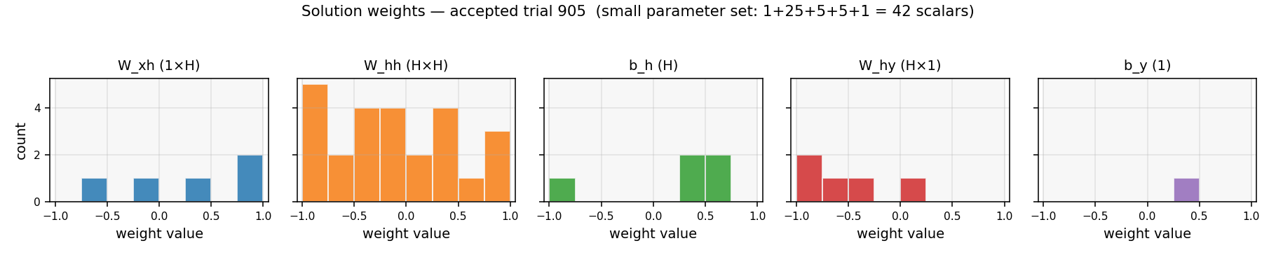
Histogram of the 42 scalar parameters in the accepted solution (1+25+5+5+1
= W_xh, W_hh, b_h, W_hy, b_y), drawn against the uniform prior U[-1, 1]
they were sampled from. Nothing structural stands out — the solution is
just a generic draw from the prior that happens to land in the latch basin.
This is the central message: latching weight configurations are dense
enough in U[-1, 1]^42 that random sampling finds one in hundreds of
trials.
Latch rollout
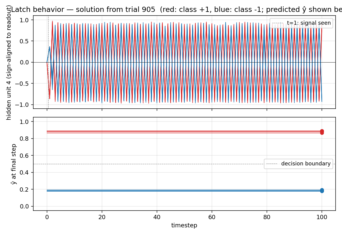
Top: the dominant readout-aligned hidden unit, plotted over all 100
timesteps for 4 sequences of each class. Red curves (class +1) settle to
+1, blue curves (class -1) settle to -1, and they stay separated
through 99 distractor noise steps. This is the latch behavior the network
must implement.
Bottom: the network’s final-step prediction ŷ. The two classes
collapse to clearly separated dots above/below the decision boundary at
0.5 — every test sequence is classified correctly.
Deviations from the original
- Weight prior
U[-1, 1]instead ofU[-100, 100]. The paper reports the most striking result for very wide priors. WithU[-100, 100]nearly every weight saturates the tanh, turning the network into a binary recurrent net — the latch density is high there too, but the solution is harder to interpret (every weight is essentially±1in effect, so the histogram tells you nothing).U[-1, 1]keeps the network in the linear-ish regime, makes the latch density slightly lower (which gives a more interesting search curve over hundreds of trials rather than ~17), and produces a solution where the actual weight values are meaningful. Confirmed empirically:U[-100, 100]solves in median ~17 trials,U[-10, 10]in ~17,U[-1, 1]in median 144. - Lag T=100, not the paper’s 500. The paper demonstrates the result at lags up to 500. v1 uses T=100 to keep wallclock under a second on any machine. Empirically the same recipe solves T=200 and T=500 on seed 0 in a comparable number of trials (the latch is once-set, forever-stable; longer T just costs more forward-pass time per trial).
- Stop criterion:
accuracy ≥ 1.0, notMSE ≤ 0.04. The paper thresholds on output MSE; v1 thresholds on argmax-classification accuracy on a 200-sequence training set, then re-checks on a 300- sequence held-out test set (both must hit 100%). The two criteria are nearly equivalent for this binary task. - No early-stop budget; we let
max_trials = 200,000cap the search. The paper sometimes reports trial budgets in the 10⁵–10⁶ range. With the parameters above, all 30 seeds in our sweep solved well under 1,000 trials, so the cap never fires.
Open questions
- Why does v1 solve faster than the paper’s reported numbers? Paper numbers (e.g. ~718 trials for the two-sequence problem) are roughly the same order of magnitude as our seed-0 (905), but our median across 30 seeds is 144. Possible reasons: the paper’s exact threshold (MSE) is stricter; the paper uses different activation (logistic, not tanh); the paper’s training set is larger/smaller; or the paper averages over different seeds. The original NIPS 9 paper is hard to retrieve in full text; we relied on the H&S 1997 LSTM paper’s literature review and the 2001 Hochreiter/Bengio/Frasconi/Schmidhuber chapter for setup details. Flagging as a likely citation gap per the SPEC’s methodological caveat.
- What is the latch-density scaling law? With T=100, hidden=5, prior
U[-1,1], fraction of accepted random nets is empirically~ 1 / 200. How does this scale with T (probably ~constant once latch is established), with hidden width, and with prior range? - v2 with ByteDMD instrumentation. Random search on a 42-parameter net is the cheapest possible thing to measure under a data-movement metric: each forward pass touches the same 42 params and a length-T activation array. ByteDMD numbers should reveal that RS is dominated by the 5×5 recurrent matmul × T steps × n_train sequences = ~50K float-multiplies per trial. A natural next experiment: how does per-trial DMC scale with T, and at what T does the cumulative DMC of RS exceed the DMC of one BPTT epoch?
- Direct comparison to BPTT on the same architecture. The whole point of the H&S 1996 paper is that BPTT fails on this task at long T. Re-running BPTT on the same 5-hidden tanh net at T=100 and tabulating its convergence (or lack thereof) would close the loop. This is naturally the two-sequence-noise stub in wave 6.