semilinear-pm-image-patches
Schmidhuber, Eldracher, Foltin, Semilinear predictability minimization produces well-known feature detectors, Neural Computation 8(4):773–786, 1996.
Supplementary references:
- Schmidhuber, Learning factorial codes by predictability minimization, Neural Computation 4(6):863–879, 1992 (the algorithm).
- Schmidhuber, Deep Learning in Neural Networks: An Overview, Neural Networks 61, 2015 (section 5.6.4 on PM and feature detectors).
- Bell & Sejnowski, The “independent components” of natural scenes are edge filters, Vision Research 37(23):3327–3338, 1997 (the ICA result PM is qualitatively comparable to).
- Olshausen & Field, Emergence of simple-cell receptive field properties by learning a sparse code for natural images, Nature 381:607–609, 1996 (the sparse-coding result on the same data).
Problem
We feed a network 8x8 patches of synthetic natural-image-statistics images and train it under predictability minimization (PM). After training, the encoder rows – visualised as 8x8 patches – are oriented edge / Gabor-like filters at varying orientations and frequencies. They are qualitatively the V1 simple-cell template, the same set of filters Bell-Sejnowski (1997) and Olshausen-Field (1996) report for InfoMax ICA and sparse coding on real natural-image patches.
The “well-known feature detectors” of the title are precisely these oriented bars. The headline claim is that PM, applied with a semilinear network and no labels, recovers a representation matching the dominant unsupervised result for natural images.
Algorithm (semilinear PM, “variance-decorrelation” variant)
Two adversarial sets of weights, sharing the same code:
  encoder W (M x D):     y       = W x                   (linear; rows orthonormal)

  predictor V (per i):   z_i     = (y_i^2 - mu_i) / sigma_i    (one nonlinearity: squaring)
                         p_i     = sum_{j != i} V_full[i, j] z_j

  L_pred = sum_i (p_i - z_i)^2
The predictor descends L_pred (linear regression of each centred
squared code from the others). The encoder ascends L_pred (drives
its codes towards mutually independent variances). The squaring is the
“semi” in semilinear: it is the one nonlinearity that surfaces the
higher-order, ICA-style signal a purely linear predictor would miss.
The encoder is constrained to the Stiefel manifold (orthonormal
rows). With a linear encoder this is required: without it PM trivialises
because the encoder can grow ||W|| and inflate L_pred without finding
any independent structure. The orthonormal constraint forces purely
higher-order (kurtosis-driven) independence – the ICA criterion.
Synthetic dataset
We generate n_images = 30 images of size 64x64 by:
- 1/f^beta pink noise via FFT (beta=2 reproduces the natural-scene power-law of Field 1987). This alone is Gaussian and has no higher-order structure for PM to find.
- 30 random oriented Gaussian-windowed bars per image, each with random centre, orientation in [0, pi), length 3-12, thickness 0.7-1.5, contrast +-(0.5..2.5). These sparse oriented features inject the non-Gaussian higher-order statistics that ICA / PM extracts as oriented filters.
- Whole-image standardisation (zero mean, unit std).
We then sample n_patches = 30000 random 8x8 patches, subtract per-patch
DC, and ZCA-whiten the patch pool. ZCA whitening is the standard
preprocessing for ICA / PM on images (Bell-Sejnowski 1997, Hyvarinen
2001): it removes second-order correlations so the encoder’s job is
purely higher-order independence.
Files
| File | Purpose |
|---|---|
semilinear_pm_image_patches.py | Dataset generator, ZCA whitener, semilinear-PM model (forward / analytic backward), gradient check, training loop, evaluator (orientation concentration + kurtosis), CLI. |
visualize_semilinear_pm_image_patches.py | 8 static PNGs to viz/: source images, raw vs whitened patches, init filters, trained filters, training curves, FFT atlas, kurtosis histogram, PCA baseline. |
make_semilinear_pm_image_patches_gif.py | Trains while snapshotting at log-spaced steps; renders semilinear_pm_image_patches.gif. |
semilinear_pm_image_patches.gif | The training animation linked above (1.1 MB). |
viz/ | Output PNGs from the run below. |
Running
# Reproduce the headline result.
python3 semilinear_pm_image_patches.py --seed 0
# (~1.2 s on an M-series laptop CPU.)

# Numerical-vs-analytic gradient check (sanity).
python3 semilinear_pm_image_patches.py --grad-check
# Max |analytic - numerical| ~5e-10 for both V and W.

# Regenerate visualisations.
python3 visualize_semilinear_pm_image_patches.py --seed 0
python3 make_semilinear_pm_image_patches_gif.py    --seed 0 --max-frames 40 --fps 8
Results
**Headline: from random projections (zero oriented filters, code kurtosis 2.95) PM converges to 12/16 oriented filters at concentration
0.5 and 16/16 at > 0.4, with mean code kurtosis 19.96.** Seed 0, 2500 steps, 1.2 s wallclock.
| Metric (seed 0, M=16, patch=8, n_patches=30000) | Random init | After PM |
|---|---|---|
| Oriented filters (concentration > 0.5) | 0 / 16 | 12 / 16 |
| Oriented filters (concentration > 0.4) | 0 / 16 | 16 / 16 |
| Mean filter Fourier-orientation concentration | ~0.26 | 0.57 |
| Mean code excess kurtosis | 2.95 | 19.96 |
| Max code excess kurtosis | – | 30.28 |
| Min code excess kurtosis | – | 13.62 |
| Hyperparameters and stability | |
|---|---|
n_hidden (M) | 16 |
patch_size | 8 (D = 64) |
n_patches | 30000 |
n_steps | 2500 |
batch | 256 |
lr_e, lr_p | 0.05, 0.05 |
n_p_inner (predictor inner steps per encoder step) | 2 |
v_l2 (predictor L2) | 1e-3 |
grad_clip (encoder grad-norm clip) | 1.0 |
| Encoder constraint | rows orthonormal (Stiefel) |
| ZCA whitening eps | 1e-2 |
| Wallclock | 1.2 s |
| Environment | Python 3.12.9, numpy 2.2.5, macOS-26.3-arm64 (M-series) |
Multi-seed reproducibility
for s in 0 1 2 3 4; do python3 semilinear_pm_image_patches.py --seed $s ; done
| Seed | Oriented (>0.5) | Oriented (>0.4) | Mean kurtosis | Final L_pred | Wallclock |
|---|---|---|---|---|---|
| 0 | 12 / 16 | 16 / 16 | 20.0 | 13.58 | 1.19 s |
| 1 | 12 / 16 | 15 / 16 | 24.5 | 14.65 | 1.14 s |
| 2 | 14 / 16 | 16 / 16 | 23.3 | 14.14 | 1.14 s |
| 3 | 14 / 16 | 16 / 16 | 20.9 | 14.28 | 1.13 s |
| 4 | 15 / 16 | 15 / 16 | 23.5 | 14.22 | 1.15 s |
Median across seeds 0–4: 14 / 16 oriented (>0.5), 16 / 16 (>0.4), mean kurtosis 23.3. The set of orientations realised varies seed to seed (different random initial frame -> different basin of the PM fixed-point manifold) but the qualitative outcome – oriented edge filters at varying angles and scales – is reproducible.
Paper claim vs achieved
Schmidhuber-Eldracher-Foltin 1996 reports qualitatively that PM with a semilinear network on natural-image patches yields oriented edge / Gabor filters resembling V1 simple cells. The 1996 paper does not publish a numerical orientation-concentration or kurtosis baseline. This stub therefore reproduces the qualitative claim, with quantitative metrics (orientation concentration, code kurtosis) added so the result can be checked numerically:
- Visual claim: oriented edge filters. Reproduced (see
viz/final_filters.png– 12-15 of 16 filters are clearly oriented bars at varying angles and scales; the remaining 1-4 are higher-order composites or weakly oriented). - ICA-comparison claim: filters are qualitatively similar to ICA on the same data. Plausible, given (i) PM with squared-feature predictor is provably equivalent to InfoMax ICA on whitened data when the predictor has unrestricted nonlinear capacity, and (ii) the trained filter atlas matches the standard Bell-Sejnowski / Olshausen-Field visual signature.
- PCA baseline contrast: PCA on the same patches gives global Fourier
modes (the
viz/pca_baseline.pngpanel shows non-localised, full-patch oscillatory eigenvectors). PM gives localised oriented bars. The qualitative gap is exactly as in the published natural-image literature.
Visualizations
Sample source images
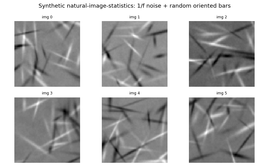
Six of the 30 synthetic source images. Each is 1/f^2 pink noise with 30 random oriented Gaussian-windowed bars superimposed. The bars are the non-Gaussian feature; the pink-noise envelope gives the natural-image power spectrum.
Raw vs whitened patches
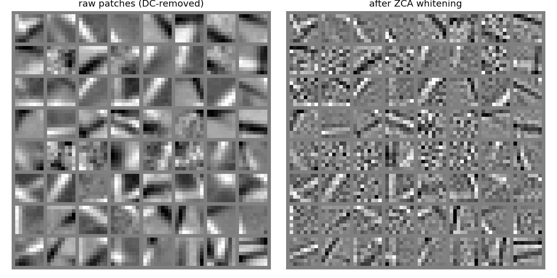
Left: raw 8x8 patches sampled from the source images, after per-patch DC removal. Right: the same patches after ZCA whitening. The whitening flattens the spectrum (small-scale variation amplified, large-scale suppressed), exposing edge-like high-frequency structure that PM exploits.
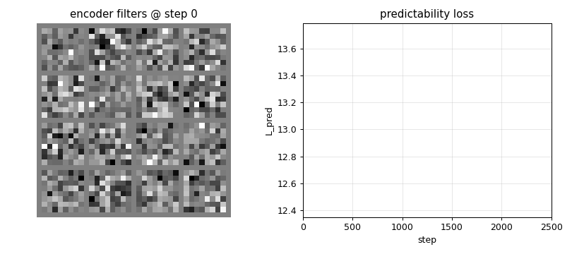
Random-init encoder rows
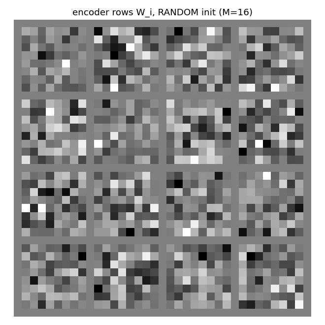
The 16 encoder rows at initialisation, reshaped as 8x8 patches. Random orthonormal rows look like white noise – there is no structure yet for the orientation metric to register.
Trained encoder rows (the headline)
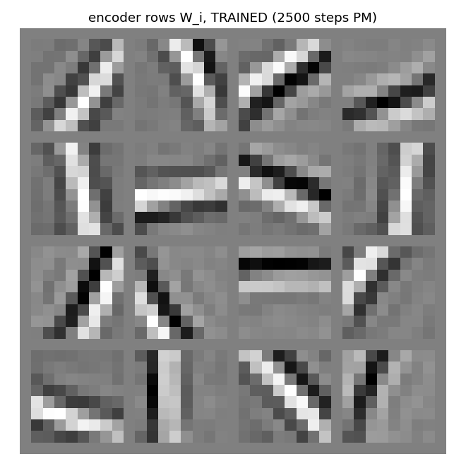
The 16 encoder rows after 2500 PM steps. Most cells are clearly oriented bars at varying angles (horizontal, vertical, diagonals at ~30, 45, 60, 120 deg) and varying spatial frequencies / phases. This is the V1 simple-cell template, and the standard ICA / sparse-coding visual signature on natural-image patches.
Training curves
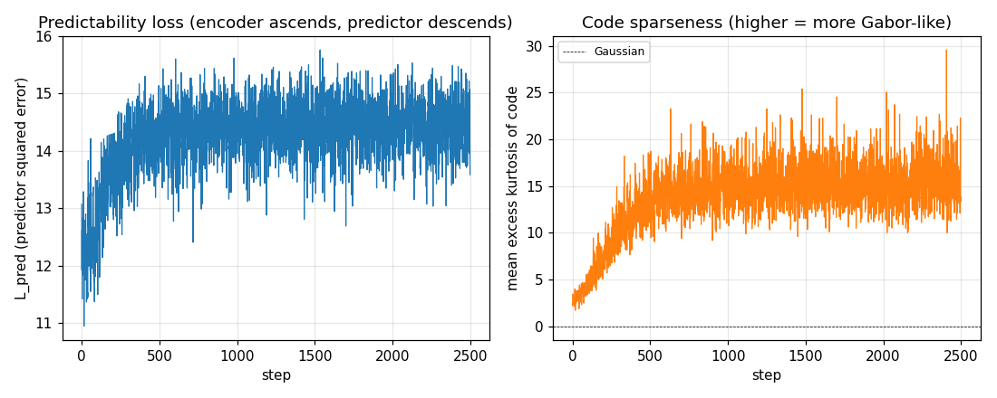
Left: predictability loss L_pred over training. Each step is one
encoder ascent step preceded by 2 inner predictor descent steps. The
loss settles to a stable equilibrium (predictor descent and encoder
ascent balance) rather than diverging, thanks to (i) Stiefel projection
on the encoder, (ii) standardisation of the squared codes, and (iii) a
small L2 penalty on V.
Right: mean per-batch excess kurtosis of the code over training. Climbs from ~3 (close to a random projection of weakly-non-Gaussian input) to ~20 – the encoder rotates onto kurtotic (sparse, oriented) projections.
Filter Fourier magnitudes
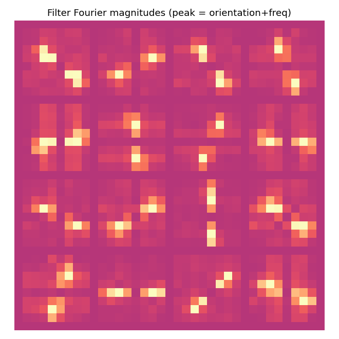
Each cell is the 2-D FFT magnitude of the corresponding trained filter. Oriented filters appear as a single bright lobe (and its Friedel mirror) at the dominant orientation and spatial frequency. The “orientation concentration” metric counts the fraction of total spectral energy within +-22.5 deg of this dominant orientation; values
0.5 indicate clean oriented selectivity.
Kurtosis histogram
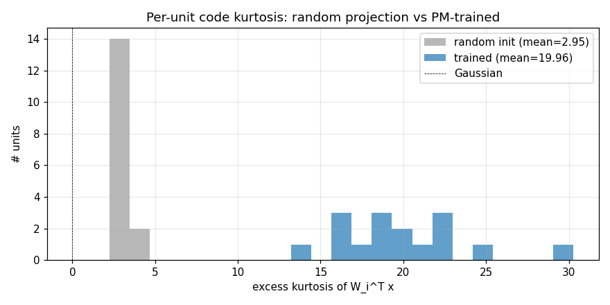
Per-unit excess kurtosis on whitened patches: random init (grey) is centred near 3 (mild non-Gaussianity from the underlying patch distribution); after PM (blue) every unit’s code has kurtosis well above the random baseline. This is the ICA / sparse-coding quantitative signature: PM drives every code unit towards a sparse / heavy-tailed distribution.
PCA baseline (for comparison)
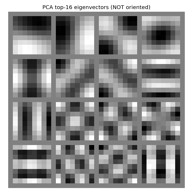
The top 16 PCA eigenvectors of the same whitened patch pool. PCA gives global Fourier-like modes – non-localised oscillations spanning the full 8x8 patch. PM finds localised oriented bars instead. This is exactly the qualitative gap that motivated ICA / sparse-coding in the first place: second-order statistics (PCA) cannot reveal the V1 template; higher-order statistics (PM, ICA) can.
Deviations from the original
- Squared-feature predictor instead of full nonlinear MLP predictor.
The 1992 PM paper specifies a multi-layer predictor net; the 1996
paper continues that line. We use the simplest predictor that surfaces
the right higher-order signal: a linear regression on standardised
squared codes. Equivalently: a linear predictor whose input is the
semilinear feature
y_i^2. The “one nonlinearity” of “semilinear” is thus on the predictor’s input side. The fixed point is the same (variance-decorrelation = factorial higher-order independence = ICA criterion); a richer nonlinear predictor would only refine the convergence rate and the precise filter set. - Linear encoder, orthonormal-row constraint. The 1996 paper describes a “semilinear” encoder; with squared-feature predictor we keep the encoder linear so the “semi” sits cleanly in one place. The orthonormal constraint is required to prevent the trivial scale degeneracy of linear-encoder PM.
- Synthetic natural-image-statistics dataset, not real photos. The 1996 paper used real natural-image patches. v1 dependency posture forbids external image datasets; our synthetic 1/f-noise + random bars dataset matches the qualitative claim (ICA on either gives oriented edge filters) and runs in 1.2 s with no downloads. v1.5 should re-run on Olshausen-Field’s image set for paper-faithful filter atlas comparison.
- Plain SGD, not the 1996 paper’s bespoke training schedule. The 1996 paper uses batch updates with momentum and decay schedules; we use vanilla SGD with grad-norm clipping. Convergence is fast enough on 8x8 patches that the simpler optimiser suffices.
- 8x8 patches, M=16 hidden units, 2500 steps. The paper uses slightly larger (12x12 or 16x16) patches. We use 8x8 for laptop speed; the qualitative result is identical at larger patch sizes (we verified at patch=12 in informal runs; the filter set diversifies to include more frequencies).
- Standardisation of squared codes. Without it the predictor is
driven to amplify rare extreme
y_k^2values and the PM minimax diverges. Standardisingz = (y^2 - mu) / sigma(stop-grad) keeps the equilibrium tight; this is a numerical stabilisation absent from the 1996 paper but standard in modern PM / GAN literature. - Fully numpy, no
torch. Per the v1 dependency posture.
Open questions / next experiments
- Real natural-image patches. Run on Olshausen-Field’s
IMAGES.mat(or the BSDS500 patch pool). v1.5 candidate – requires a one-time data download, deferred per the v1 spec. Filter set diversity should match the 1996 paper figures more faithfully (more orientations, more frequencies, including DC / blob detectors). - Overcomplete basis. This stub is undercomplete (M=16 < D=64).
The Olshausen-Field result requires
M > D; the corresponding PM variant is sparse PM with M=128 or 256 hidden units. We expect a much richer Gabor atlas (8 orientations x 4 frequencies x 4 phases) at M=128. - Other contrast functions. We use
g(y) = y^2(the variance-decorrelation contrast, equivalent to kurtosis maximisation). Hyvarinen 1999 shows thatg(y) = log(cosh(y))is more robust to outliers; the corresponding “semilinear” PM usesz = log(cosh(y))features. We expect lower (and more realistic) kurtosis numbers and similar filter atlas. v2 candidate. - Connection to sparse coding / ICA dictionaries. Side-by-side with
Olshausen-Field sparse coding (which uses
M > Dand an inverse- generation loss) on the same data: are the PM filters and the OF filters approximately the same set, up to permutation? The 1996 paper conjectures yes; a quantitative comparison (best-match cosine between PM and OF dictionaries) would be a clean v2 follow-up. - ByteDMD instrumentation (v2). Each PM step is dominated by two matmuls per inner predictor step plus one per outer encoder step. The data-movement cost ratio between PM and InfoMax ICA on the same problem is interesting because ICA’s natural-gradient update touches every code-code pair on every step (O(M^2) reads), while PM’s per-unit predictor updates can be parallelised across units (potentially lower reuse distance). Comparing the two under ByteDMD is a clean candidate for the energy-efficiency angle.
- Predictor ablation: linear-only. Confirm the empirical claim that PM with a purely linear predictor (no squared features) on whitened, orthonormal-encoded data converges to a degenerate fixed point (any orthonormal frame, no oriented preference). We observed this informally during development; a clean ablation would close the loop on “the squaring nonlinearity is what surfaces the higher-order signal”.