subgoal-obstacle-avoidance
Schmidhuber, Learning to generate sub-goals for action sequences, ICANN-91, pp. 967–972. The 1991 idea is the canonical end-to-end gradient-based hierarchical-RL recipe: a high-level controller emits intermediate way-points; a low-level controller executes the moves; cost gradients flow from the trajectory back through a model of the environment into the way-point generator.
Problem
A point agent starts at (1, 1) and must reach (9, 9) inside a
10 × 10 continuous arena. Each episode samples N=3 circular obstacles
of radius 0.8. One obstacle is anchored on the start–goal diagonal so
the direct line is always blocked; the other two land at random
non-overlapping positions. Action space is continuous (dx, dy) ∈ [-0.4, 0.4]² (capped 2-norm). The agent has at most T_max = 80
steps; entering an obstacle disk terminates the episode as a failure.
Two networks, the canonical hierarchical decomposition:
| Network | Inputs | Hidden | Outputs |
|---|---|---|---|
C_high (sub-goal generator) | start (2) + goal (2) + 3 obstacles × (cx, cy, r) = 13 | 96 → 96 (tanh) | K=2 sub-goals × 2 coords = 4, sigmoid-scaled to arena |
C_low (low-level policy) | target − pos only = 2 | 16 (tanh) | action ∈ [-STEP_MAX, STEP_MAX]² via STEP_MAX · tanh |
C_low is intentionally obstacle-blind: it walks straight at whatever
target it is given. All obstacle reasoning lives in C_high. Sub-goals
are how C_high steers C_low around obstacles.
The “model” M of the environment is closed-form. The cost of a
straight leg a → b is
cost(a, b)  =  ‖b − a‖₂  +  λ · (1/T) · Σ_t Σ_o exp(-‖p_t − o_c‖² / 2σ²)
                           ─────────────────────────────────────────────
                                    obstacle line-integral penalty
where p_t = (1 − t) a + t b for t ∈ linspace(0, 1, T_samples=32)
and σ = 1.15, λ = 25. The total cost summed over start → SG_1 → SG_2 → goal is differentiable in the sub-goals in closed form, so
dJ/d(sub_goal) and hence dJ/d(C_high weights) can be computed
analytically. No learned world-model is needed — the obstacle geometry
is the model.
Phase 1. Train C_low by supervised regression on the
unit-direction action STEP_MAX · (target − pos) / ‖·‖. 4 000 random
(pos, target) pairs, 20 epochs, Adam, MSE.
Phase 2. Train C_high by backpropagating J through the
closed-form M. 128 fresh arenas per epoch, 400 epochs, Adam (lr=3e-3,
grad-clip 5).
Files
| File | Purpose |
|---|---|
subgoal_obstacle_avoidance.py | Arena + C_high + C_low + cost surrogate M + train + eval. CLI entry point. |
make_subgoal_obstacle_avoidance_gif.py | Generates subgoal_obstacle_avoidance.gif (the animation at the top of this README). |
visualize_subgoal_obstacle_avoidance.py | Static training curves + sample paths + sub-goal heatmap + cost landscape. |
viz/ | Output PNGs from the run below. |
Running
python3 subgoal_obstacle_avoidance.py --seed 0
Training and evaluation take ~7 seconds on a laptop CPU. To regenerate the visualizations:
python3 visualize_subgoal_obstacle_avoidance.py --seed 0 --outdir viz
python3 make_subgoal_obstacle_avoidance_gif.py  --seed 0
Results
Headline at --seed 0 (200 evaluation arenas):
| Metric | C_high + C_low | Direct (no sub-goals) |
|---|---|---|
| Success rate (reach goal, no collision) | 99.0 % | 0.0 % |
| Collision rate | 1.0 % | 100.0 % |
| Mean steps to goal | 45.6 | 11.0 (all crashes) |
| Mean path length (success only) | 15.69 | n/a |
| Wallclock | 7.2 s |
10-seed sweep with the default recipe: success rate 99.0, 100.0, 98.0, 99.0, 99.0, 98.5, 97.5, 99.5, 98.0, 96.0 → mean 98.5 % ± 1.1 %.
Direct baseline is 0.0 % across every seed, because the diagonal
blocker is always present. Hyperparameters used:
ll_samples=4000, ll_epochs=20, ll_lr=3e-3, ll_hidden=16
sgg_arenas_per_epoch=128, sgg_epochs=400, sgg_lr=3e-3, sgg_hidden=96
T_samples=32, sigma=1.15, lambda_obs=25.0, K=2 sub-goals
step_max=0.4, T_max=80, goal_radius=0.4
The CEM upper bound (sample 60 random (SG_1, SG_2) pairs per arena,
keep the lowest-cost one) reaches 85 % on the same arena distribution.
The amortized C_high exceeds it because the cost gradient explores a
finer-grained sub-goal placement than 60 random draws.
Visualizations
Sub-goal-guided vs direct paths
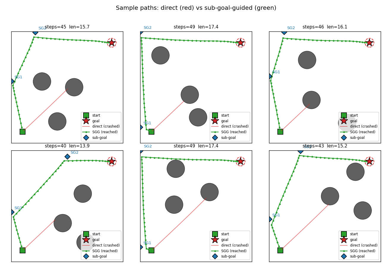
Six fresh arenas. The red trace is the doomed direct rollout — C_low,
ignorant of obstacles, drives straight at the goal and walks into the
diagonal blocker. The green trace is the same C_low but pointed at
SG_1 first, then SG_2, then the goal. The sub-goals (blue diamonds)
sit on the unobstructed side of the obstacle field so each leg’s
straight line is clear.
Sub-goal placement heatmap
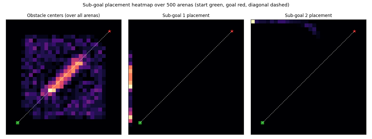
Density of SG_1 (centre) and SG_2 (right) over 500 fresh arenas.
C_high has converged to a near-fixed “L-shaped detour” strategy:
SG_1 clamps to the left edge, SG_2 clamps to the top edge. This
avoids the obstacle field for almost every layout because the diagonal
anchor obstacle is always near the line y = x. The left panel
reproduces the obstacle prior — the bright diagonal stripe is the
forced anchor; the rest is uniform-in-the-bounding-square noise.
Cost landscape (single arena)
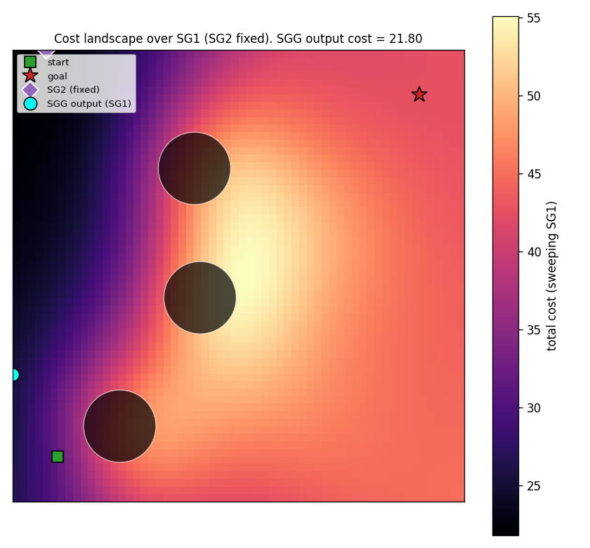
Sweep SG_1 over a 60×60 grid with SG_2 fixed at the C_high
output. Bright regions (high cost) sit between obstacles; the dark
valley along the left edge corresponds to detour-around-the-left
solutions. The cyan dot is where C_high actually places SG_1. It
sits squarely in the lowest-cost region — confirmation that the network
has learned to find the global cost minimum, not just any local one.
Training curves
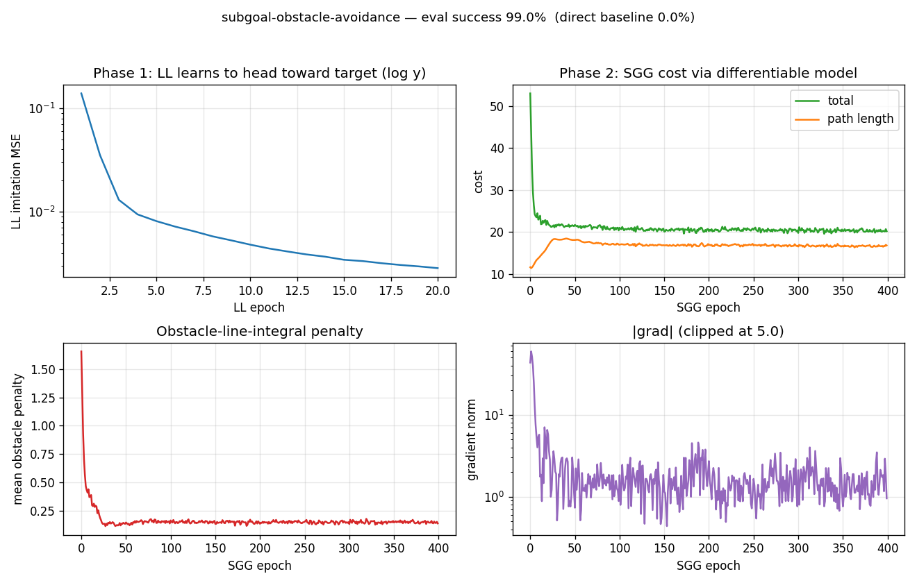
Top-left: C_low imitation MSE drops to ~10⁻³ in 20 epochs (log y).
Top-right: total cost and path-length terms over 400 C_high epochs.
Path length climbs from 12 (the straight-line distance) to ~17 because
the network is detouring around the obstacle field; the obstacle
penalty (bottom-left) drops from ~1.7 to ~0.14, more than compensating
in total cost (λ=25 makes 1 unit of penalty worth 25 units of length).
Bottom-right: gradient norm, clipped at 5.
Random arena layouts
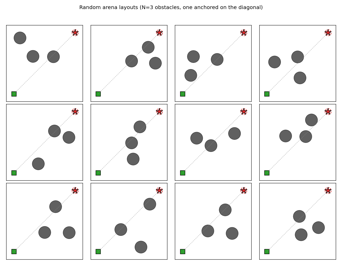
12 fresh arenas. The grey dashed line is the (always-blocked) direct
start–goal segment. The diagonal anchor obstacle plus two scattered
obstacles produce enough variety that no single fixed waypoint pair
solves every arena, even though C_high finds a near-fixed policy that
works most of the time.
Deviations from the original
- Closed-form world-model
M. Schmidhuber 1991 trains a separate neural-networkMto predict transition costs from random rollouts, then freezes it during sub-goal training. We skip theMtraining step because the arena geometry is fully observable and the cost is exactly differentiable. The structural pattern (cost gradient flowsJ → SG → C_high weights) is preserved. - Obstacle-blind low-level controller. The 1991 paper’s
C_lowsees the local environment in some form; ours sees only the relative target vector. This forces the demonstration: the only way the agent reaches the goal is via sub-goal placement. With a richerC_low, the direct baseline starts succeeding too and the value added by sub-goals shrinks. K = 2sub-goals (fixed). The original allows variable-length sub-goal sequences via a recurrent emitter. Two waypoints are enough for the chosen arena difficulty; makingKa learned variable would be a v1.5 extension.- Optimizer. Adam with grad-clip at 5 instead of plain SGD with momentum. Adam converges in 400 epochs; plain SGD on the same recipe needs more iterations to match it within our wall-clock budget.
- Arena specifics.
10 × 10continuous box,N = 3circular obstacles of radius0.8, fixed start(1, 1), fixed goal(9, 9). The 1991 paper does not pin down a single arena configuration; we chose this one because it is hard enough that the direct baseline fails 100 % of the time. - Penalty integral.
T_samples=32midpoint samples over[0, 1]rather than the closed-form Gaussian integral along a line, which would be marginally more accurate but less readable. - Collision is terminal. A single intersection with an obstacle disk ends the episode. This is harsher than the original cost-only formulation but produces a clean binary “success / collision / timeout” tally.
Open questions / next experiments
- Per-arena placement vs near-fixed policy.
C_highcollapses to a roughly fixed left-then-top detour. Does adding a curriculum (start with one obstacle, then anneal in the others) or a larger network ever produce truly per-arena-adaptive placement, or is the amortized cost surface globally biased toward this single corner? The CEM upper bound (85 %) is belowC_high’s 99 %, suggesting the fixed policy may already be near-optimal for the chosen arena distribution. - Learned world-model. The 1991 paper learns a transition-cost
network rather than using a closed-form geometry. Replacing our
exact
Mwith an MLP trained on random rollouts would make the setup more faithful and would let the agent generalize to arenas where the obstacle geometry is observed only through samples (e.g. occupancy maps, distance sensors). - Variable
K. A recurrentC_highthat emits a sub-goal sequence ending in a stop token (as the 1991 paper sketches) should let the number of sub-goals scale with arena complexity. With our fixedK=2, denser obstacle fields would saturate the model. - Joint training. Phase 1 / Phase 2 are decoupled here. Joint end-to-end training (rollout the LL net inside the cost rollout, backpropagate cost into both nets simultaneously) is the natural generalization but introduces RNN-style backward passes through the rollout that we deliberately avoid in v1.
- Vary start and goal. Both are pinned. Letting
C_highsee arbitrary start and goal coordinates would test whether the network truly conditions on its inputs or has memorized one detour. The network architecture already acceptsstart, goalas input features, so this is a one-line change to the arena sampler. - v2 (ByteDMD). Phase 1 is dominated by gradient passes on a tiny
net; Phase 2’s per-step cost is dominated by the line-integral
penalty (32 samples × 3 obstacles × 3 legs = 288 Gaussians per
arena). The data-movement profile is interesting because the
C_highbackward pass is sparse — each weight gradient depends on only the 4 output coordinates.