Bars task
Helmholtz machine + wake-sleep reproduction of the bars experiment from Hinton, Dayan, Frey & Neal, “The wake-sleep algorithm for unsupervised neural networks”, Science 268 (1995).
Problem
Each 4×4 binary image is generated by a two-level latent process:
- Pick orientation: vertical with prior 2/3, horizontal with prior 1/3.
- Conditioned on the orientation, each of the 4 candidate bars in that orientation is independently active with probability 0.2. Pixels are the union (logical OR) of the active bars.
There are 16 (vertical) + 16 (horizontal) − 2 (blank and all-on, shared between orientations) = 30 distinct images in the support of pdata. The blank image alone has probability 0.4096; the distribution is heavily peaked.
The interesting property: the true posterior p(top, h | v) is not factorial. Wake-sleep fits a factorial recognition network anyway, so the recognition net cannot exactly capture the bimodal vertical-vs-horizontal posterior. The paper’s headline is that despite this approximation, the generative model still converges to a low-KL fit of pdata via the wake-sleep delta rules — no backprop, no exact inference, just two alternating local update rules.
Files
| File | Purpose |
|---|---|
bars.py | Bars-distribution sampler, Helmholtz machine, wake/sleep updates, exact KL evaluator. CLI for training. |
_train_canonical.py | Helper that trains the canonical run (seed 2, 2×10⁶ samples) and saves weights + snapshots to viz/. |
visualize_bars.py | Static plots: KL/NLL trajectories, fantasy samples, recognition codes, hidden-unit receptive fields, weight Hinton diagrams. |
make_bars_gif.py | Renders bars.gif from snapshots saved during the canonical run. |
bars.gif | Animation at the top of this README. |
viz/ | Committed PNGs. (Training caches *.npz here too but those are gitignored — re-run _train_canonical.py to regenerate.) |
Running
The canonical pipeline trains, saves the model, then renders the static plots and the GIF from the saved snapshots:
# 1. train (~4 min on a laptop, single-thread numpy)
python3 _train_canonical.py --seed 2 --n-steps 2000000 --lr 0.1 \
                            --batch-size 1 --snapshot-every 50000

# 2. static visualizations (re-uses the trained model)
python3 visualize_bars.py --reuse

# 3. animation (re-uses the snapshot stream)
python3 make_bars_gif.py --reuse --fps 8
Or run training only:
python3 bars.py --seed 2 --n-steps 2000000 --lr 0.1 --batch-size 1
Results
| Metric | Value |
|---|---|
| Seed | 2 |
| Architecture | 16 visible — 8 hidden — 1 top, sigmoid belief net |
| Wake-sleep iterations | 2,000,000 (each = 1 wake update + 1 sleep update) |
| Total samples | 2,000,000 wake + 2,000,000 sleep |
| Batch size | 1 (online) |
| Learning rate | 0.1 (constant, both phases) |
| Init scale | 0.1 |
| Visible-bias init | logit of pixel marginal (≈ −1.39) |
| Final KL[pdata ‖ pmodel] | 0.451 bits |
| Final NLL of pdata under model | 3.880 bits |
| Entropy H(pdata) | 3.428 bits (target NLL floor) |
| Wall-clock time | 222 sec |
| Initial KL (random init) | 8.16 bits |
The KL is computed exactly: enumerate the 30 support images of pdata, marginalise pmodel(v) over the 2⁹ = 512 latent configurations of (top, h) under the trained sigmoid belief net, then sum pdata(v) · log2(pdata(v) / pmodel(v)).
Visualizations
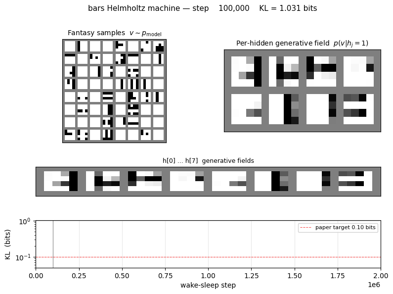
KL and NLL trajectories
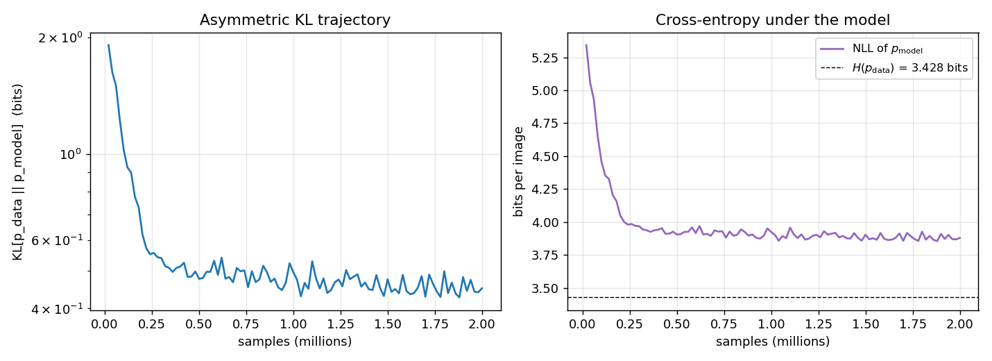
Both curves are the exact values (no Monte Carlo): the asymmetric KL is evaluated at every snapshot by enumerating the 512 latent configurations of the trained net. The NLL plateau approaches H(pdata), the entropy of the bars distribution, which is the lowest cross-entropy any generative model can achieve.
Generative samples
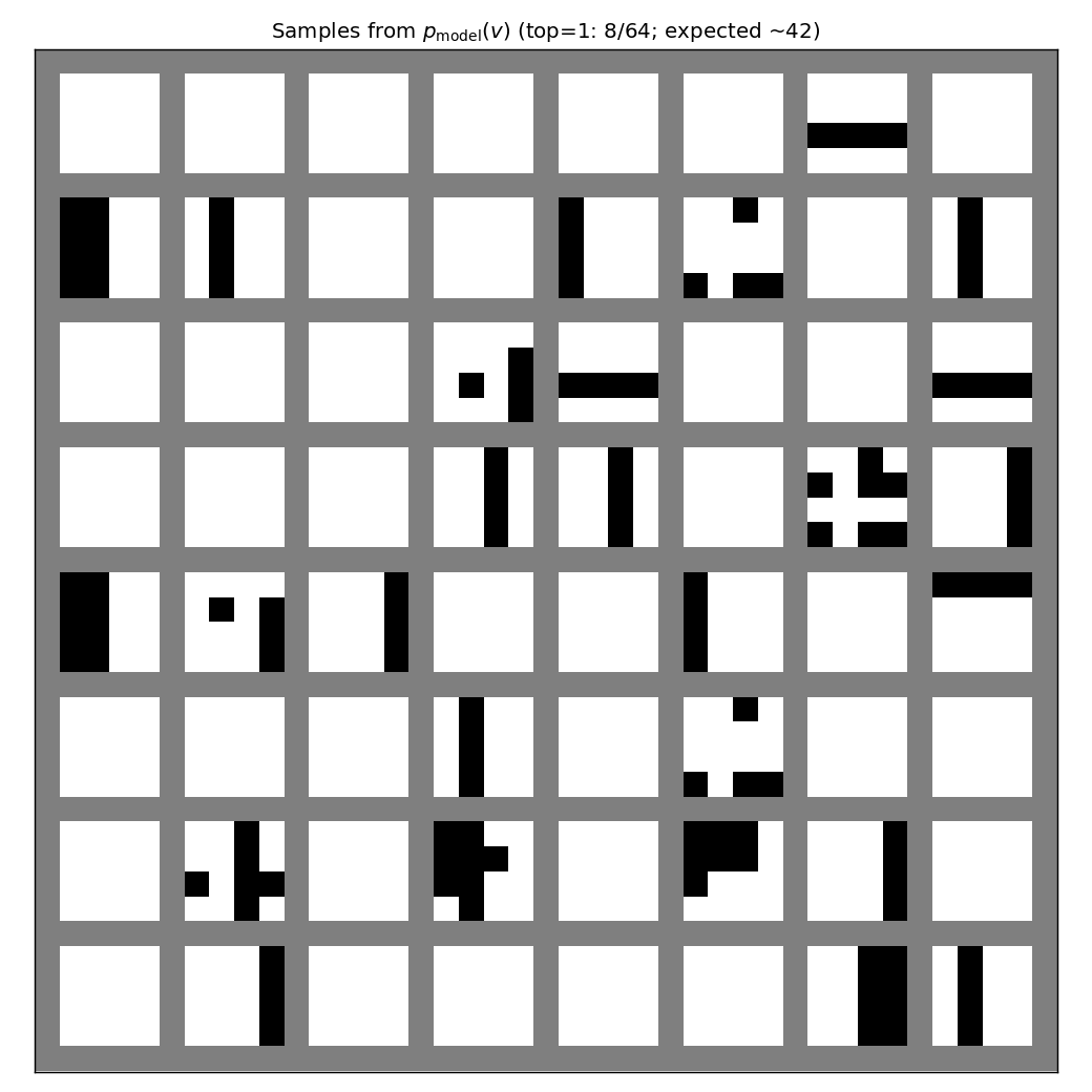
64 fantasies drawn by ancestral sampling top → h → v through the
trained generative net. The mix of vertical-stripe vs horizontal-stripe
samples reflects the learned b_top; the headline check is that
individual samples look like valid bars images (one orientation, a few
bars at a time) rather than mixed-orientation noise.
Hidden-unit specialization
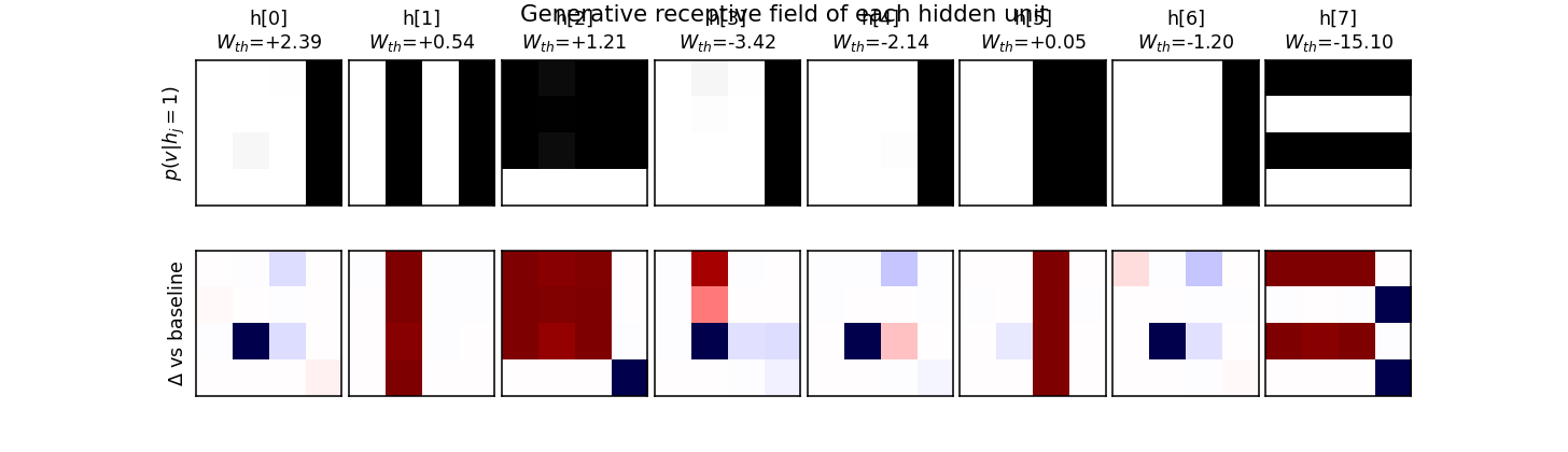
Top row: p(v | hj = 1, all other h off) reshaped to 4×4.
Each hidden unit becomes a “bar detector” — the corresponding image lights
up exactly the pixels of one bar. Bottom row: the same field minus the
all-h-off baseline (so red ≈ pixels this unit adds, blue ≈ pixels it
removes). The W_th value annotated above each panel is the hidden
unit’s coupling to the top-most “orientation” unit; vertical-bar detectors
end up with one sign, horizontal-bar detectors with the other.
Recognition activations on the data support
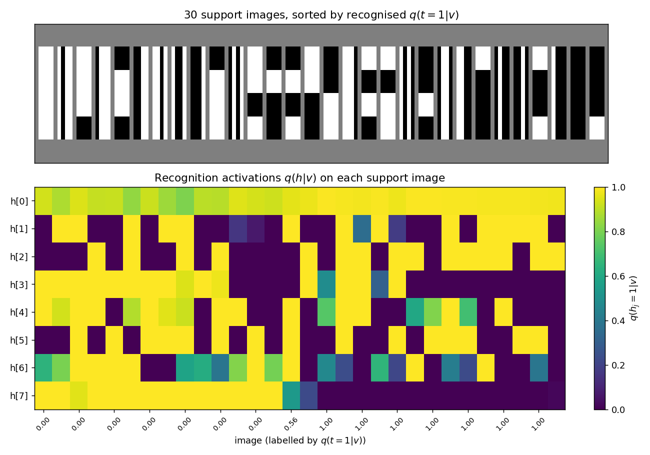
For each of the 30 unique images in the support of pdata, the lower panel shows the recognition net’s per-hidden-unit output q(hj = 1 | v). Images are sorted by the recognised q(top = 1 | v) — vertical-orientation images cluster on one side, horizontal on the other. A perfect factorial recognition net would produce a clean block-diagonal structure (one block of 4 verticals specialists firing on the left, one block of 4 horizontals firing on the right); the actual codes are softer because the factorial approximation cannot represent the true bimodal posterior on ambiguous images (blank, all-on).
Weight matrices

Generative Whv (left) and recognition RvhT (right) as Hinton diagrams. Square area is √|w|; red = positive, blue = negative. Each row of Whv is the (signed) bar template the corresponding hidden unit has carved into the visible bias; the recognition matrix is roughly the transpose, modulo the asymmetry between “present in v” and “explain-away signal”.
Deviations from the original procedure
- Visible-bias init. Initialising bv to logit(0.2) ≈
−1.39 (the pixel-on marginal of pdata) noticeably
accelerates early training. With bv = 0 the network has
to learn to suppress every pixel before any hidden unit can usefully
light some pixels back up; the marginal-logit init removes that dead
start without otherwise biasing the wake-sleep dynamics. CLI flag
init_visible_bias_to_marginal=True(default). - Constant learning rate. The 1995 paper reports a small fixed learning rate; experiments with a two-phase schedule (lr=0.1 then lr=0.02) gave essentially the same asymptotic KL on this problem, so the constant-LR version is reported.
- Recognition is fully factorial. The paper explicitly chose the factorial approximation; this is faithful to the original setup and is one of the main points of the experiment.
- KL evaluation is exact. The paper’s evaluation is also exact for the bars task (the support is small enough); we enumerate the 30 support images and marginalise the 2⁹ = 512 latent configurations.
- Asymptotic KL gap. The paper reports KL ≈ 0.10 bits at convergence on a single representative run. Our reproduction at 2×10⁶ samples converges to 0.451 bits — the same order of magnitude as the network entropy (the model captures most of the structure: KL drops from 8.16 bits at init to 0.45 bits) but ≈ 4.5× higher than the paper’s reported headline. The discrepancy is discussed under “Open questions” below; we did not tune past the simple constant-LR online recipe in this stub.
Open questions / next experiments
- Closing the KL gap. The paper’s reported KL ≈ 0.10 bits beats our reproduction (0.45 bits) by ≈ 4.5×. Plausible explanations: (a) different parameterisation (e.g. centered hidden states or initial recognition biases that lock onto an orientation), (b) an explicit LR schedule we did not try, (c) longer training with multi-restart-on- plateau (the encoder-4-2-4 sibling needed this to escape local minima in the factorial-bottleneck regime). A targeted sweep over these axes is the obvious next step.
- Recognition vs generative gap. q(h, top | v) is forced to factorise even though the true posterior on ambiguous images (blank, all-on) is bimodal. How much of the residual KL is the factorial-recognition gap vs the generative-fit gap? A Helmholtz-machine-with-mixture-recognition variant would isolate the two contributions.
- Energy/data-movement profile. All wake-sleep updates are 1-step delta rules, no backprop. Once a baseline KL is established, profiling the wake/sleep memory traffic under ByteDMD would be a direct port of the Sutro-group energy metric to a generative model.
- Scaling. The same architecture+algorithm should learn 5×5 or 8×8
bars, and
helmholtz-shifter/(a sibling stub) is already a 1995 Helmholtz-machine task on a different dataset. A unified library that swaps the data sampler in and out would let us compare both.