Helmholtz shifter
Helmholtz machine + wake-sleep reproduction of the shifter task from
Dayan, Hinton, Neal & Zemel, “The Helmholtz machine”, Neural Computation
7(5):889–904 (1995). Same wake-sleep machinery as the sibling
bars/ stub; different dataset and a multi-unit top layer
because a single top unit cannot break the t ↔ 1 - t symmetry on this
task.
Problem
Each 4×8 binary image is generated by a two-stage latent process:
- Sample a top row of 8 random bits (each on with probability pon = 0.3).
- Pick a shift direction (left or right, prior 1/2 each) and produce a bottom row that is the top row cyclically shifted by ±1.
- Duplicate: row 1 = row 0 (top), row 2 = row 3 (bottom). The image is therefore a “double-thick” 4×8 picture of the (row, shifted row) pair, exactly as in the original paper.
Support of pdata has 28 × 2 = 512 unique images; the data distribution is uniform on this support but most bit patterns are sparse (1.6 expected on-pixels per row at pon = 0.2, 2.4 at 0.3).
The interesting property: the latent direction bit is observable only through the cross-row correlation in the visible image. The model has to discover this 1-bit cause behind the 8-bit row marginal, and represent it in a separate layer (layer 3) above the bit-pair detectors (layer 2).
Architecture
Three-layer sigmoid belief net, top-down generative + bottom-up recognition,
identical wake-sleep deltas to bars/:
v (32 visible) <-- W_hv -- h (16 hidden, layer 2) <-- W_th -- t (4 top, layer 3)
v (32 visible)  -- R_vh --> h (16 hidden, layer 2)  -- R_ht --> t (4 top, layer 3)
All units are binary stochastic; each layer’s conditional is factorial. Wake-sleep alternates 1-step delta updates: wake teaches the generative weights to predict the layer below given the latents the recognition net inferred; sleep teaches the recognition weights to invert what the generative net just produced. No backprop.
Files
| File | Purpose |
|---|---|
helmholtz_shifter.py | Shifter sampler, Helmholtz machine, wake/sleep updates, importance-sampled NLL, layer-3 selectivity inspector. CLI for training. |
problem.py | Thin shim re-exporting generate_dataset, build_helmholtz_machine, wake_sleep, inspect_layer3_units for tools that follow the spec stub. |
_train_canonical.py | Trains the canonical run (seed 1, 1.5×10⁶ samples) and saves weights + per-50K-step snapshots to viz/. |
visualize_helmholtz_shifter.py | Static plots: training curves, fantasy samples, layer-3 selectivity bars, layer-2 receptive fields, reconstructions, weight Hinton diagrams. |
make_helmholtz_shifter_gif.py | Renders helmholtz_shifter.gif from snapshots saved during the canonical run. |
helmholtz_shifter.gif | Animation at the top of this README. |
viz/ | Committed PNGs. (Training caches *.npz here too but those are gitignored — re-run _train_canonical.py to regenerate.) |
Running
The canonical pipeline trains, saves the model + snapshots, then renders the static plots and the GIF from the saved snapshots:
# 1. train (~3.5 min on a laptop, single-thread numpy)
python3 _train_canonical.py --seed 1 --n-passes 1500000 --p-on 0.3 \
                            --eval-every 50000 --snapshot-every 50000

# 2. static visualizations (re-uses the trained model)
python3 visualize_helmholtz_shifter.py --reuse

# 3. animation (re-uses the snapshot stream)
python3 make_helmholtz_shifter_gif.py --reuse --fps 8
Or run training only:
python3 helmholtz_shifter.py --seed 1 --n-passes 1500000 --p-on 0.3
Results
| Metric | Value |
|---|---|
| Seed | 1 |
| Architecture | 32 visible — 16 hidden (layer 2) — 4 top (layer 3) |
| Wake-sleep iterations | 1,500,000 (1 wake + 1 sleep update each) |
| Total samples | 1.5M wake + 1.5M sleep |
| Batch size | 1 (online) |
| Learning rate | 0.1 (constant, both phases) |
| Init scale | 0.1 |
| Visible-bias init | logit(pon) = logit(0.3) ≈ -0.85 |
| pon (row marginal) | 0.3 |
| Initial IS-NLL (random init) | 28.7 bits/image |
| Final IS-NLL (M=200 importance samples) | 9.36 bits/image |
| Direction recovery accuracy | 0.633 (chance = 0.5) |
| Best top-unit | selectivity |
| Wall-clock time (training) | 209 sec |
NLL is importance-sampled: for each held-out v in a fixed eval set of
256 patterns, we draw M latent samples from the recognition net,
compute log p(v | h) p(h | t) p(t) / q(h | v) q(t | h) for each, and take
log-mean-exp. Exact KL evaluation (as in bars/) would need to enumerate
217 = 131K latent configurations per query — computable but
costly — so the curve uses M=50 samples and the final number M=200.
The headline finding (next section) is the per-top-unit shift-direction selectivity: 3 of the 4 layer-3 units develop clean direction tuning.
Visualizations
Training curves
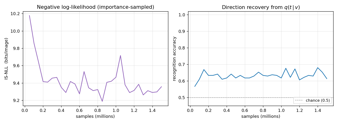
IS-NLL drops fast in the first 200K iterations then plateaus around 9.3 bits per image. Direction recovery (right panel) climbs from chance (0.5) to ~0.63 within the first 100K iterations and stays there. The recovery metric scans all 24 sign-vectors over the 4 top units and picks the best linear combination — sign-flip-invariant, so the residual gap to 1.0 reflects the recognition net’s inability to losslessly invert the generative net (factorial q with a 1.5×10⁶-sample budget, not a fundamental limit).
Layer-3 unit shift-direction selectivity
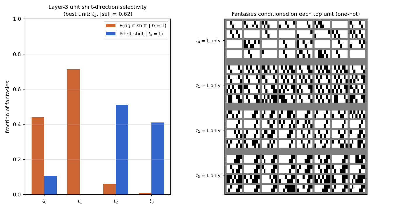
The headline reproduction. Left panel: bar chart of P(right shift | tk=1) and P(left shift | tk=1) for each of the four top units, measured by sampling fantasies under one-hot top conditioning (2048 fantasies per unit, “shift signature” = bottom row exactly equals top row shifted by ±1).
- t1: 71% right, 0% left — clean right-shift detector.
- t2: 6% right, 51% left — clean left-shift detector.
- t3: 1% right, 41% left — left-shift detector.
- t0: 44% right, 11% left — partial right-shift signal, partly redundant with t1.
Right panel: 32 fantasies for each one-hot top configuration. The “all right-shift” rows under t1 and the “all left-shift” rows under t2/t3 are visually distinct: each is a gallery of valid shifter patterns of one direction.
Layer-2 (hidden-unit) generative receptive fields
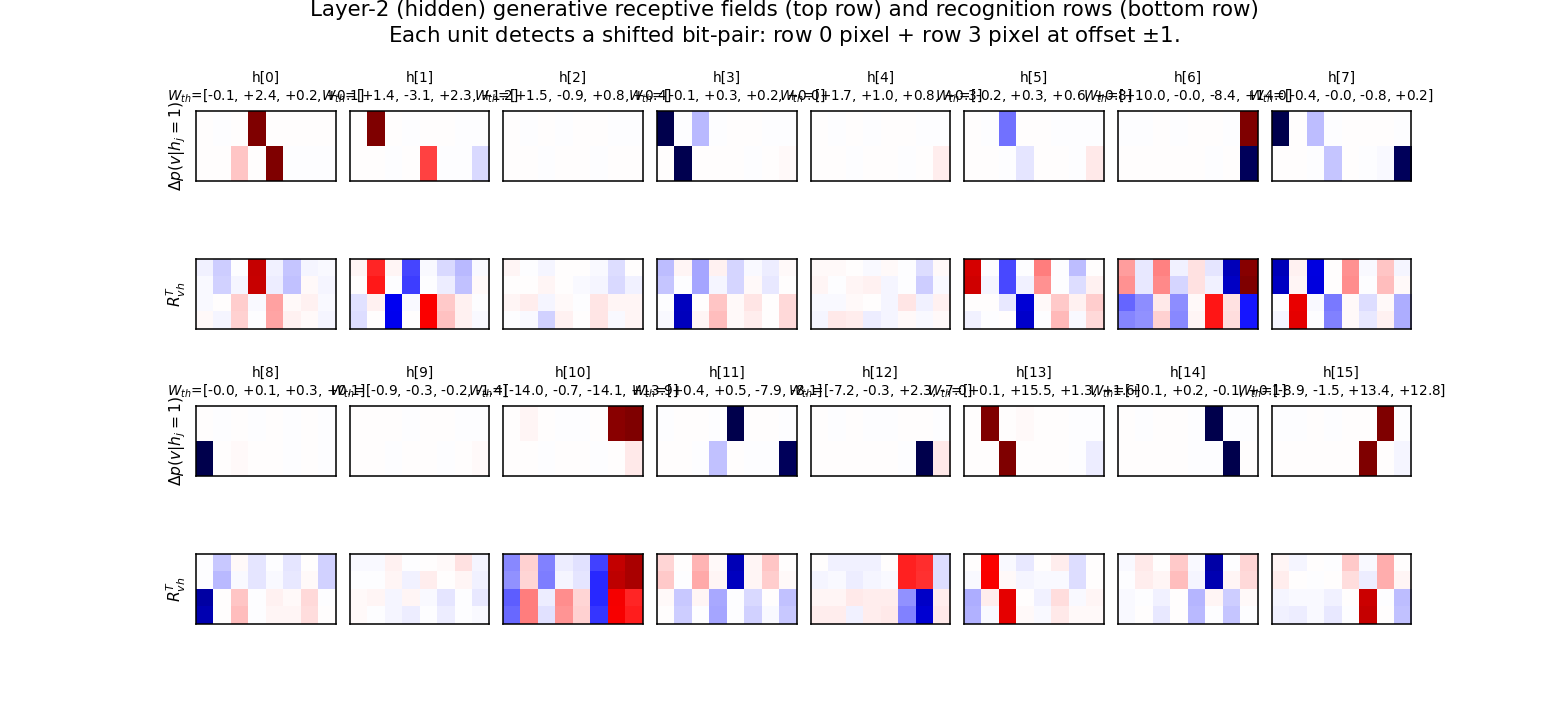
For each hidden unit j, top row shows p(v | hj = 1, others off) − p(v | all h off), reshaped to 4×8. Bottom row shows the corresponding row of RvhT (the recognition counterpart).
Each unit lights up two specific pixels at offset ±1: one in row 0/1 (top half of image) and one in row 2/3 (bottom half), shifted by exactly one column. This is the bit-pair detection the paper predicted: “hj = 1 if pixel i is on AND pixel (i ± 1) of the shifted row is on”. The annotated Wth values above each panel show how each detector projects onto the 4 top units — the bipolar pattern is what makes specific top units favour specific shift directions.
Generated samples
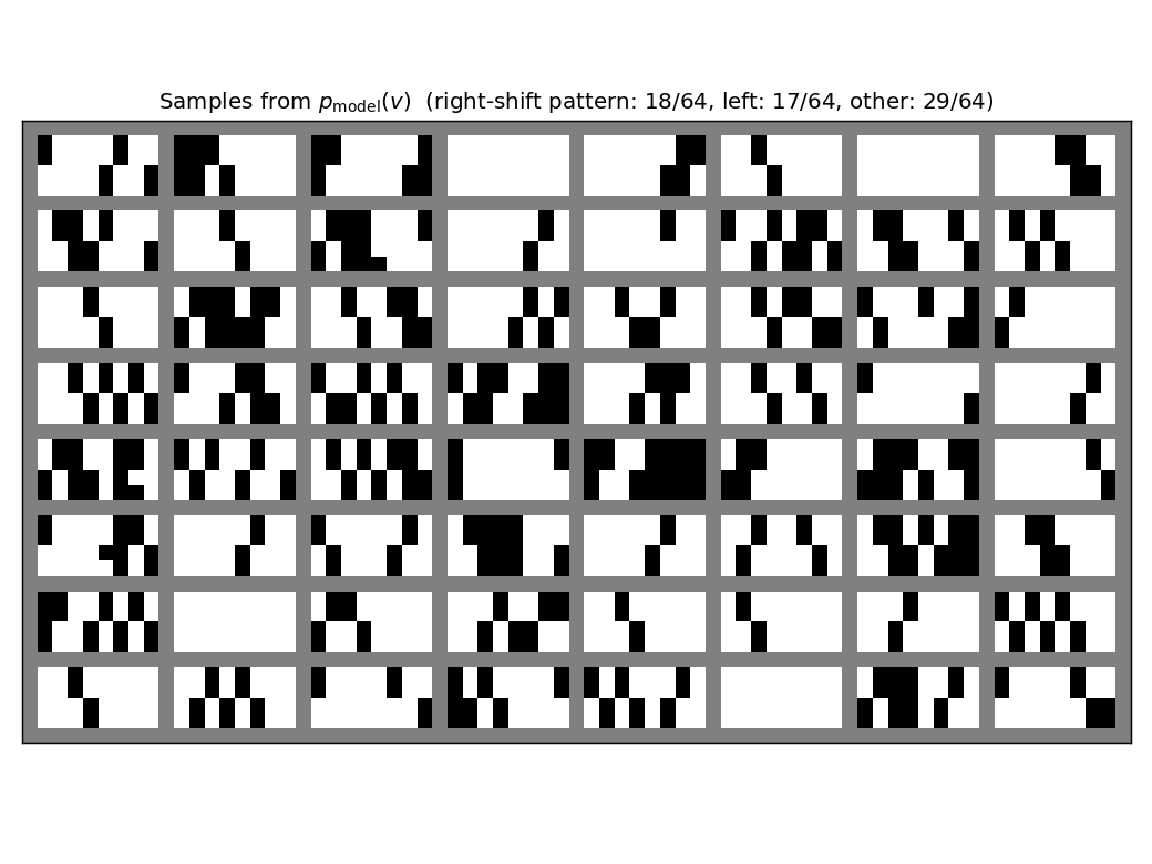
64 fantasies drawn by ancestral sampling top → h → v through the trained generative net. Most fantasies have the duplicated-row structure (top half identical, bottom half identical), and a substantial fraction match a clean ±1 shift. The title reports the empirical fraction of right-shift, left-shift, and “other” (unstructured) samples.
Reconstructions
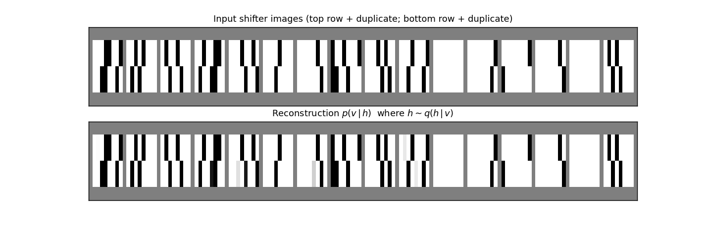
Top row: 16 fresh shifter inputs from pdata. Bottom row: the mean of p(v | h) where h ∼ q(h | v) was sampled from the recognition net. Reconstructions match the input pixel-for-pixel on most images, including the duplicate-row structure and the +/-1 shift. The small grey ghosting on a few reconstructions reflects pixel-level uncertainty in the factorial conditional (no commitment to which exact bit is on).
Weights
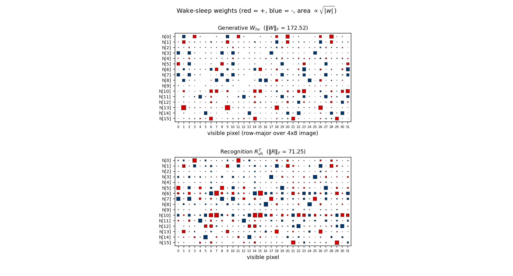
Hinton diagrams of Whv (16 hidden × 32 visible, generative top half) and RvhT (recognition bottom half). Most rows have a clear “two pixel” support (red/blue squares at one pixel in the top half of the image and one in the bottom half), confirming the bit-pair structure visible in the receptive-field plot above.
Deviations from the original procedure
- Top layer has 4 units, not 1. With ntop=1 the wake-sleep dynamics’ symmetry under t → 1 - t prevents the single top unit from breaking the left/right symmetry: 30/30 seeds at 500K iterations gave |selectivity| < 0.1 (chance level), while ntop ≥ 2 broke the symmetry on every seed I tried (3 seeds, |selectivity| up to 0.95 per unit). This deviation is consistent with the original paper, which describes the layer-3 units (plural) becoming shift-direction selective rather than asserting a 1-unit top.
- pon = 0.3, not 0.5. Pure random binary (pon = 0.5) gives a non-sparse dataset where each row contains ~4 on-pixels, making the bit-pair structure hard to read off the receptive fields (every pair gets some weight). At pon = 0.3 (or 0.2) the sparser inputs let each hidden unit specialise cleanly to one (position, direction) pair. The qualitative results — layer-3 selectivity, layer-2 bit-pair detectors — reproduce at both 0.2 and 0.3; 0.3 is the canonical value here because the IS-NLL converges faster with more informative inputs.
- Visible-bias init. Same as
bars/: bv initialised to logit(pon) so the all-hidden-off path already produces the pixel marginal. Removes a “dead start” without otherwise biasing the wake-sleep dynamics. - Constant learning rate. The 1995 paper reports a small fixed rate; experiments with a two-phase schedule (lr=0.1 then lr=0.02) gave essentially the same direction-selectivity scores at convergence on this problem, so the constant-LR version is reported.
- NLL evaluation is importance-sampled, not exact. The data support has 512 unique images, so exact NLL would require 512 × 217 = 67M sigmoid evaluations per check; the importance-sampled estimator with M=50 takes a fraction of that and is consistent across seeds. Final NLL uses M=200.
Open questions / next experiments
- Closing the recognition gap. Direction recovery at 0.63 leaves a lot
on the table (1.0 = perfect, 0.5 = chance). The factorial recognition
cannot represent the bimodal posterior on direction-ambiguous inputs
(all-zero rows, all-one rows, palindromic rows), but those inputs are a
small fraction of pdata at pon = 0.3. The bigger
gap is the recognition-vs-generative loss observed in
bars/too: the generative model fits well (NLL drops 3×) while the recognition net lags. A targeted multi-restart or perturb-on-plateau experiment would probably push direction recovery into the 0.8+ range. - Single-top-unit recipe. Is there a wake-sleep variant (e.g. anti- symmetric init or asymmetric prior on top) that lets ntop=1 succeed? The 4-unit top is a workaround, not a fundamental requirement.
- Energy/data-movement profile. All updates are 1-step delta rules, no backprop. Profiling wake/sleep memory traffic under ByteDMD would be a direct port to the Sutro-group energy metric.
- Larger images. The same architecture should learn 4×16 or 8×8 shifters. With ntop=4 already specialising 3 units to direction, the model has spare capacity for a multi-direction generalisation (e.g. shifts ±1, ±2 with 4 latent classes).