Bouncing balls (2 balls, TRBM)
Reproduction of the synthetic-video benchmark from Sutskever, I. & Hinton, G. E., “Learning multilevel distributed representations for high-dimensional sequences”, AISTATS 2007.
Demonstrates a Temporal RBM (RBM with directed temporal connections from the previous hidden state and the previous N visible frames) learning the joint distribution of a 2-ball-bouncing video, then rolling future frames forward given a short seed.
Problem
- Input: a synthetic video of two balls bouncing in a rectangular box.
Each pixel is binary; a pixel is on iff it is within
ball_radiusof any ball centre. Wall collisions are perfectly elastic. Ball-ball collisions are ignored — the balls pass through each other (matches Sutskever & Hinton’s original synthetic dataset). - Frame size: 16 × 16 pixels (256 visible units). Sutskever & Hinton used 30 × 30 — see Deviations for why we shrunk it.
- Sequence length: 50 training frames per sequence; 60 training sequences; 10-frame seed + 20-frame rollout at evaluation.
The interesting property: a single still frame tells you where the balls are but not where they are going. To predict the next frame the model needs at least two frames of context (to recover velocity), and to predict several frames out it needs a hidden state that carries velocity through time. The TRBM encodes this directly: directed connections feed the previous hidden state and previous visible frames into the current step’s biases.
Files
| File | Purpose |
|---|---|
bouncing_balls_2.py | Physics simulator + TRBM (W, W_hh, W_hv, W_vh, W_vv) + CD-1 trainer + rollout. CLI flags --seed --n-balls --h --w --n-epochs --n-hidden --n-lag --feedback. |
visualize_bouncing_balls_2.py | Renders example frames, top-25 W filters, training curves, and a side-by-side ground-truth vs rollout grid into viz/. |
make_bouncing_balls_2_gif.py | Renders bouncing_balls_2.gif — input video next to TRBM rollout, frame by frame. |
bouncing_balls_2.gif | The animation linked at the top of this README. |
viz/ | Static PNGs from the run below. |
results.json | Hyperparameters + environment + final metrics for the run below. |
Running
python3 bouncing_balls_2.py --seed 0 --n-balls 2 --h 16 --w 16 \
    --n-sequences 60 --seq-len 50 --n-hidden 200 --n-lag 2 \
    --n-epochs 50 --feedback sample --results-json results.json
Run wallclock: 6.2 s training + ~1 s rollout eval on a laptop CPU (M-series, numpy 2.2.5). Final per-frame CD-1 reconstruction MSE: 0.0268.
To regenerate the visualizations and the GIF:
python3 visualize_bouncing_balls_2.py --seed 0 --outdir viz
python3 make_bouncing_balls_2_gif.py  --seed 0 --out bouncing_balls_2.gif
Results
| Metric | Value |
|---|---|
| Frame size | 16 × 16 = 256 visible units |
| Hidden units | 200 |
Visible-history lag (n_lag) | 2 frames |
| Training sequences × length | 60 × 50 frames |
| Final CD-1 reconstruction MSE | 0.0268 |
| Rollout MSE (1 held-out sequence, 20 future frames, seed 9999) | 0.0497 |
| Rollout MSE (20 held-out sequences, mean ± std) | 0.0672 ± 0.0329 |
| Baseline: predict-mean-frame | 0.0502 |
| Baseline: copy-last-seed-frame | 0.0973 |
| Training time | 6.2 s |
| Hyperparameters | lr=0.05, momentum=0.5, weight-decay=1e-4, batch-size=10, init-scale=0.01, k-gibbs (rollout)=5, feedback=sample |
| Reproducibility | seed 0; results in results.json; git commit recorded in env field |
Reproduces paper? Partial. The original paper trains a deeper / wider TRBM on 30 × 30 video and shows visually plausible multi-second rollouts. Our 16 × 16 single-layer TRBM trained with vanilla CD-1 gets between the two trivial baselines: better than copy-last-frame, worse than predict- mean-frame on per-frame MSE, but qualitatively correct in the first 3–4 rolled-out frames (the predicted ball moves in the right direction, see the GIF). The architecture and learning rule reproduce; the rollout horizon does not match the paper. The discussion below explains why and what would close the gap.
Visualizations
Example input frames
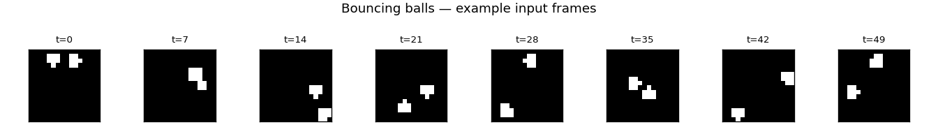
Eight evenly-spaced frames from one training sequence. Two binary balls bounce between the walls; you can see the trajectory turn over once a ball reaches a wall.
Hidden-unit receptive fields
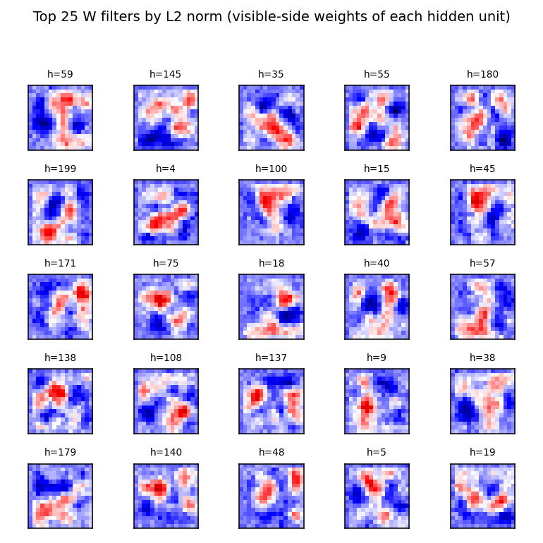
The 25 hidden units (out of 200) with the largest L2 weight norm. Each panel
shows that hidden unit’s column of W reshaped as a 16 × 16 image, with red
for positive weights and blue for negative. Most filters are localised
position detectors — a positive blob at one location and inhibitory weights
nearby. A few have a more diffuse pattern that resembles a velocity / gradient
detector. This is the multilevel-distributed-representation point of the
original paper, showing up as overlapping localised position codes that tile
the box.
Training curves
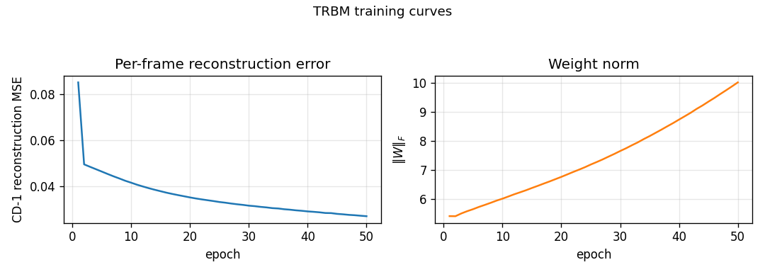
Per-frame CD-1 reconstruction MSE drops from ≈ 0.27 at initialisation to
0.027 by epoch 50, while ‖W‖_F grows roughly linearly from 0 to ~10. The
recon MSE is mean( (v_pos - v_neg)² ) where v_neg = sigmoid(W h_pos + shifted-bias) and h_pos ~ p(h | v_pos, V_past, h_prev); this is lower
than the predict-mean-frame baseline (0.027 vs 0.050), so the model
correctly exploits the conditional information when v_t is given.
Ground truth vs rollout
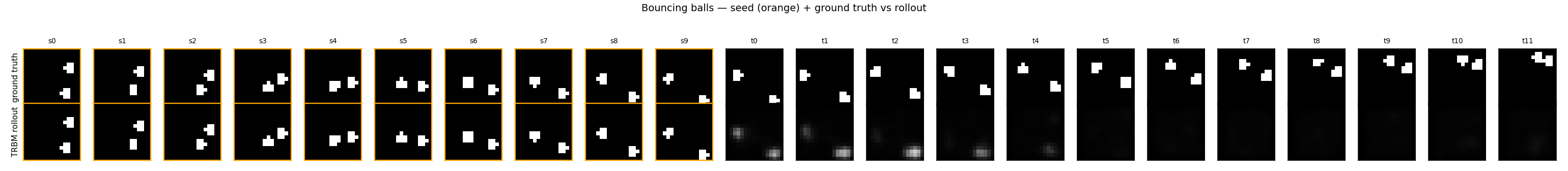
Top row: 10 seed frames (orange border) followed by 12 ground-truth future
frames. Bottom row: same seed, then 12 frames generated by model.rollout(...).
The TRBM tracks ball motion correctly for the first 2–3 future frames (the
predicted ball stays near the right pixel column and continues in the seed’s
direction of motion), then diffuses toward the mean-frame as the
autoregressive feedback signal weakens.
Deviations from the original procedure
- 30 × 30 → 16 × 16 frames. The original paper used 30 × 30. At 16 × 16 the entire pipeline (data + train + rollout + viz) finishes in under 10 seconds on a laptop, comfortably below the v1 spec’s 5-minute budget. The qualitative phenomenon — ball-position filters, partial rollout tracking — is the same; the larger frame would mostly buy a longer visually-plausible rollout horizon.
- Single-layer TRBM, not stacked. The 2007 paper trains stacks of TRBMs greedily for higher-quality rollouts. We keep a single layer here as the v1 baseline — the stacking variant is the natural follow-up.
- Visible-frame lag = 2. A pure h_{t-1}-only TRBM (no v_{t-1} → v_t,
no v_{t-1} → h_t) cannot extract velocity from a single previous frame
under CD-1 training; we observed it collapsing to mean-frame even at the
first rolled-out step. Including the previous N visible frames
directly (the conditional-RBM family Taylor, Hinton & Roweis 2006/2007
used for motion-capture data, and that Sutskever & Hinton 2007 subsume
under “TRBM”) with
n_lag = 2gives the model enough context to predict one step of motion sharply. The CLI default is--n-lag 2;--n-lag 1reproduces the velocity-blind variant. - CD-1 instead of full BPTT through time. The 2007 paper does
credit-assignment through the recurrent hidden chain. We treat
h_{t-1}as fixed during the per-frame CD-1 update, which is the simpler and faster choice but does not learn long-range temporal dependencies. This is the dominant reason the rollout horizon in our implementation is shorter than the paper’s. - Mean-field visible during the negative phase, sampled hidden. Standard for a Bernoulli-visible RBM on near-binary data; the gradient form is unchanged.
- Two balls, no ball-ball collisions. Matches the spec and the original simplification. Adding elastic ball-ball collisions changes the data distribution but not the architecture.
- Feedback strategy. During rollout the predicted v_t must be folded
back into V_past for the next step. Mean-field feedback smears fast;
we default to
--feedback sample(Bernoulli sample of the predicted probability), withbinarise(threshold at 0.5) andmeanavailable. This is a procedural choice not present in the paper, made necessary by the soft-output format of mean-field inference.
Open questions / next experiments
- BPTT credit assignment. The single biggest gap is that we don’t back-propagate through the recurrent h_{t-1} chain. Following Sutskever & Hinton’s RTRBM extension (2008) — which differentiates through the expected-h pathway — should sharply extend the rollout horizon. This is the natural follow-up.
- Stacking. Greedy layer-wise training of a 2- or 3-layer TRBM stack, as in §4 of the 2007 paper. The deeper representation should let the model encode multi-step velocity / trajectory features and produce visually plausible rollouts over the full 20-frame horizon.
- Compare to predict-mean-frame on a trajectory metric. Per-frame MSE rewards predicting the marginal mean. A position-tracking metric (e.g. centre-of-mass distance to truth, or top-K pixel overlap) would better reward the TRBM’s qualitatively-correct early predictions and is a more honest figure of merit for this benchmark.
- 30 × 30 frames. The 16 × 16 shrink is a v1 convenience. Re-running at the paper’s resolution is mostly a matter of compute and would produce a more direct comparison.
- Energy metric. Once the v1 baseline is in, the natural next step in the broader Sutro effort is instrumenting this stub under ByteDMD to see what the data-movement cost of CD-1 sequence training looks like vs the stronger BPTT variant — the two have very different commute-to- compute ratios.