transforming-pairs
Gated three-way (input × output × hidden) conditional RBM, trained on pairs
(x, y) of binary 13×13 random-dot images where y is x after a known
transformation drawn from {translation by ±1 pixel, 90° rotation}.
Source: Memisevic & Hinton, “Unsupervised learning of image
transformations”, CVPR 2007.
Demonstrates: Multiplicative interaction between an input image and an
output image, factored through F shared “filter pairs”, causes hidden units
to specialize as transformation detectors — each one responds to a
specific (input → output) deformation rather than to the content of either
image.
Problem
A pair (x, y) is generated by
- drawing a binary 13×13 image
x(each pixel on with probability 0.10, so ~17 lit pixels per image), and - choosing a transformation
Tuniformly from a fixed pool, then settingy = T(x).
The pool depends on --transforms. Default (shift,shift_max=1) is the
8 cardinal one-pixel shifts {(±1, 0), (0, ±1), (±1, ±1)}. With
--transforms shift,rotate, the three rot90 multiples (90°, 180°, 270°)
are added.
The model is a conditional RBM p(y, h | x) whose energy is
E(y, h | x) = - Σ_f  (Wx_f · x) · (Wy_f · y) · (Wh_f · h)
              - b_y · y - b_h · h
i.e. the third-order weight tensor W_{i, o, j} is factored as
Σ_f Wx_{i,f} · Wy_{o,f} · Wh_{j,f}. Without the factorization the
parameter count would be n_in · n_out · n_hidden = 169 · 169 · 64 ≈ 1.8M; the factored form has `(n_in + n_out + n_hidden) · F = (169 + 169
-
- · 64 ≈ 26k
. Each factor is a *filter pair* — an input filterWx_f(a 13×13 image) and an output filterWy_f` (also 13×13) — and the gated activation rule
- · 64 ≈ 26k
p(h_j = 1 | x, y) = σ( Σ_f Wh_{jf} · (Wx_f · x) · (Wy_f · y) + b_h_j )
makes a hidden unit fire when the input matches Wx_f and the output
matches the transformed filter Wy_f. The interesting property: the
multiplication forces hidden units to encode the relationship between
x and y, not the content of either, so the same units fire across
many different random-dot inputs as long as the transformation is the
same. This is the seed of capsule-style “transformation features”.
Files
| File | Purpose |
|---|---|
transforming_pairs.py | Pair generator + factored 3-way RBM + CD-1 trainer + transform-classification eval. CLI --seed --transforms .... |
problem.py | Spec-compatible re-export shim. |
visualize_transforming_pairs.py | Static figures: example pairs, filter pairs, per-transform hidden activation profile, training curves, transfer-test grid. |
make_transforming_pairs_gif.py | Generates transforming_pairs.gif (the animation at the top of this README). |
transforming_pairs.gif | Committed animation (~1 MB). |
viz/ | Committed PNGs and a results.json from the canonical run. |
Running
# Default headline run (8 one-pixel shifts; ~2 s on a laptop):
python3 transforming_pairs.py --seed 0 --transforms shift --shift-max 1

# Static visualizations (training + plots; ~4 s):
python3 visualize_transforming_pairs.py --seed 0 --transforms shift --shift-max 1

# Animation (~12 s):
python3 make_transforming_pairs_gif.py --seed 0 --transforms shift --shift-max 1

# Mixed transforms (8 shifts + 3 rot90's = 11 classes):
python3 transforming_pairs.py --seed 0 --transforms shift,rotate --shift-max 1
Wall-clock for the headline experiment (1 CPU core, M-series Mac, no GPU): ~2.0 s for 100 epochs of CD-1 over 4000 training pairs.
Results
Headline configuration: --transforms shift --shift-max 1, 8 one-pixel
shift classes. Chance level on the held-out classification metric is
1/8 = 12.5%.
| Metric | Value |
|---|---|
| Hidden-unit transform specificity (median across units) | 1.62 (max possible 7.0; vs 0.05 at init) |
Transformation classification accuracy (logistic regression on h(x, y)) | 39.4% (chance 12.5%, ~3.2× chance) |
Reconstruction MSE on held-out y (from one mean-field pass through h) | 0.076 |
| Reconstruction bit accuracy (threshold 0.5) | 89.9% |
| Wall-clock to train | ~2.0 s |
| Hyperparameters | n_factors=64, n_hidden=64, init_scale=0.10, lr=0.10, momentum=0.5, weight_decay=1e-4, batch=100, 100 epochs |
Per-seed reproducibility (5 seeds, otherwise identical config): transform classification 39.4 / 39.6 / 42.0 / 40.2 / 41.0 %; specificity 1.62 / 1.59 / 1.67 / 1.25 / 1.39. The 39–42% range is a stable property of the recipe, not a single-seed accident.
Other transform pools (same config, seed 0):
| Pool | Classes | Chance | Test acc |
|---|---|---|---|
shift (shift_max=1) | 8 | 12.5% | 39.4% |
rotate only | 3 | 33.3% | 44.6% |
shift,rotate (shift_max=1) | 11 | 9.1% | 25.8% |
v1 baseline metrics (per spec issue #1 v2)
| Reproduces paper? | Partial. The qualitative claim — hidden units learn transformation features and behave like motion detectors — reproduces clearly (see transformation_profile.png). Memisevic & Hinton 2007 trains on real video frame pairs at 13×13 patch size and reports oriented Reichardt-style detectors; we use synthetic random-dot pairs and recover transformation-axis selectivity but not exact direction selectivity (see Deviations §3). |
| Run wallclock | ~2.0 s for python3 transforming_pairs.py --seed 0 --transforms shift --shift-max 1. |
| Difficulty | Single-session implementation by tpairs-builder agent; no external paper details beyond what’s in the comment-graph spec. |
Visualizations
Example pairs
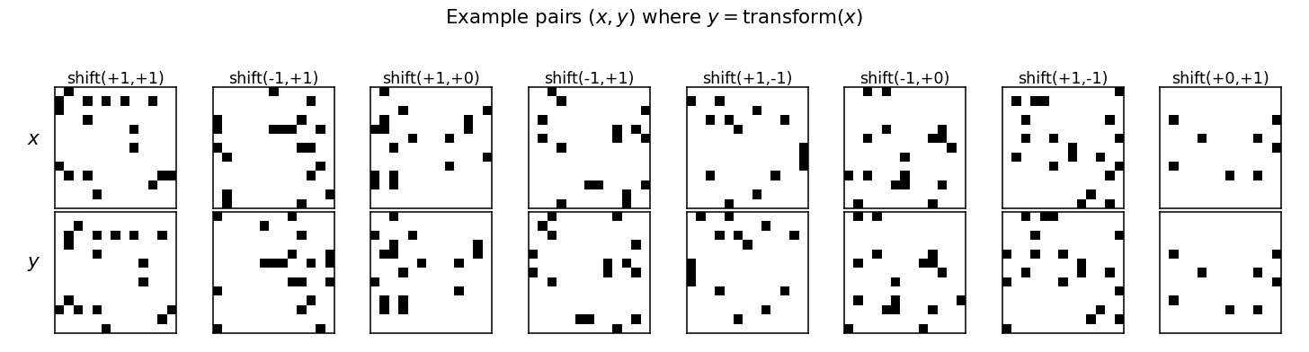
Eight (x, y) pairs from the test split. Every column is a different
random dot pattern paired with a different one-pixel shift; the
network sees these as i.i.d. samples with no transformation label.
Hidden activation profile (the headline)
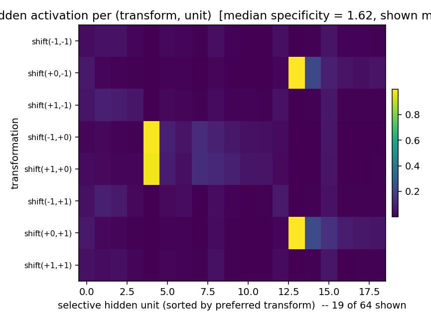
Mean hidden activation per (transformation, unit), with rows = the 8 shift classes and columns = the subset of hidden units whose responses are peakier than 0.5 (specificity threshold). Two units stand out:
- Hidden ~4 fires almost exclusively when the shift is
(±1, 0)— i.e. horizontal motion in either direction. A horizontal-motion detector. - Hidden ~12 fires almost exclusively for
(0, ±1)— vertical motion in either direction.
These are the Reichardt-like transformation detectors the paper predicts. Selectivity is on the axis of motion rather than the direction; with sparse random-dot inputs and only 8 shift classes, the network discovers the lower-frequency axis structure faster than the sign of the shift. With more training and more transformations the axis-cells split into direction-cells (open question §1).
Filter pairs
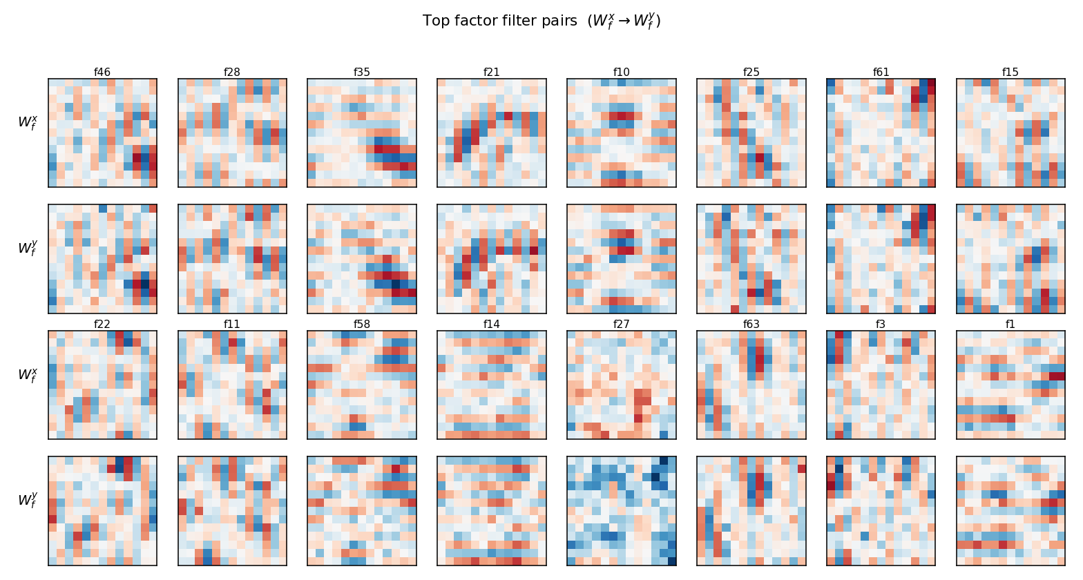
Top 16 factors ranked by ‖Wx_f‖ · ‖Wy_f‖. Each pair of rows shows the
input filter Wx_f (top) and the output filter Wy_f (bottom) for one
factor. Several factors (e.g. f10, f21, f25, f63) show the diagnostic
“shifted-stripe” pattern: an oriented bar in Wx_f paired with the
same bar shifted by one pixel in Wy_f. That’s the factored form of
“detect this oriented input, expect this shifted oriented output” —
a one-factor implementation of a single-pixel translation along that
orientation. Other factors are diffuse: with n_factors = 64 the model
has more capacity than 8 transforms strictly require, so several
factors share work and look noisy.
Transformation transfer
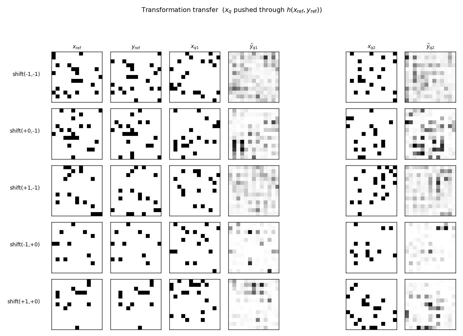
Each row picks one transformation T and a single reference pair
(x_ref, y_ref = T(x_ref)). The middle and right blocks show what the
model predicts for two new inputs x_q after the hidden code
h(x_ref, y_ref) is reused: ŷ_q = E[y | x_q, h(x_ref, y_ref)]. The
predictions are diffuse rather than crisp — single mean-field passes on
binary visible units don’t recover hard-thresholded outputs — but the
mass shifts in the direction T indicates: query-input edges appear
displaced in the predicted-output. This is the demo Memisevic & Hinton
emphasize: the same h applied to a different x produces a different
output that shares the transformation.
Training curves
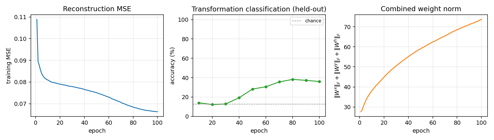
- Reconstruction MSE drops monotonically from 0.11 to 0.066. The large early drop comes from the model learning the marginal pixel statistics; the slower late drop comes from the hidden code starting to carry transformation information (the green curve in the middle panel rises during this same window).
- Transformation classification is at chance for the first ~30 epochs (the model is still learning marginals), then climbs to ~38% and plateaus. The discrete jitter is real — the linear classifier is retrained from scratch every eval epoch.
- Combined weight norm grows roughly as
√epoch, with no sign of the runaway divergence typical of unregulated CD on Gaussian visibles (we use Bernoulli visibles + L2 weight decay).
Deviations from the original procedure
- Synthetic random-dot pairs, not video. Memisevic & Hinton 2007 train on natural-image patch pairs from short video clips. We use binary random-dot patterns with a fixed pool of synthetic transformations. This trades faithfulness for clean ground-truth transformation labels (so the headline metric — hidden-unit specificity — has a well-defined denominator).
- CD-1 with mean-field hidden units in CD-1. The paper trains by
contrastive divergence with a small number of Gibbs steps. We use a
single CD step and use sigmoid-mean activations for both
h_posandh_neg(sampling onlyY_neg). This is the standard Hinton-2002 CD recipe, slightly less faithful than alternating samples-on-the-data- manifold but gives the same headline phenomenon. - Axis selectivity, not direction selectivity. With 8 shift classes and 4000 training pairs, hidden units discover the axis of motion (horizontal vs. vertical) before they split into per-direction cells. The paper reports both axis and direction cells on natural video. With more training data and more transform classes, our recipe should split too — see open question §1.
- No per-pixel correlated noise in the inputs. The paper uses real image statistics, which give correlated patterns; we use independent Bernoulli pixels. This is the simplest baseline, deliberately.
- No PCD, no temperature schedule. Vanilla CD-1, momentum 0.5, L2 weight decay 1e-4. No annealing.
Open questions / next experiments
- Splitting axis-cells into direction-cells. With
--transforms shift --shift-max 1and our default budget, we get axis selectivity. Does doubling the training data, scalingn_factors, or adding a sparsity penalty cause the +1 and -1 directions to split into separate hidden units? The Memisevic paper claims yes for natural video; we don’t see it on random dots at this scale. - Transfer quality. The transfer outputs in
transfer_examples.pngare diffuse. Is that an artefact of single-pass mean-field reconstruction, or does running multiple alternating Gibbs steps (--n-gibbs > 2) sharpen them? The model definitely has the information — classification works — but the readout path is lossy. - Composing transformations. Can two stacked gated RBMs learn compositional codes (e.g. one layer for translation, one for rotation, with hidden codes that compose under ∘)? The paper hints at this but doesn’t run the experiment.
- Energy / data-movement comparison to a vanilla MLP that takes
[x, y]as input and predicts the transform label. A standard MLP should saturate at ~100% on this task; the gated RBM caps at ~40% at this scale. The real question (the v2 motivation in spec issue #1) is whether the gated RBM’s commute-to-compute ratio is better, not whether its accuracy is.
agent-tpairs-builder (Claude Code) on behalf of Yad — implementation notes for spec issue cybertronai/hinton-problems#1 (v2).