Bouncing balls (3 balls, RTRBM)
Source: Sutskever, I., Hinton, G. E., & Taylor, G. W. (2008/2009), “The recurrent temporal restricted Boltzmann machine,” NIPS 21.
Demonstrates: A Recurrent Temporal RBM (RTRBM) — an RBM whose hidden
bias at time t is shifted by W_h r_{t-1} — can model continuous video
of three balls bouncing in a box. The recurrent matrix W_h is the only
structural addition over a per-frame RBM.
Problem
- Visible: 30 × 30 = 900 binary pixels (anti-aliased disks rendered by the simulator; values in [0, 1]).
- Hidden: 100 binary hidden units.
- Recurrent: a 100 × 100 hidden-to-hidden matrix
W_h. This is the only structural difference between an RTRBM and a per-timestep RBM. - Sequences: 30 sequences of length 100 generated fresh per run by a Newtonian simulator (3 balls, radius 3, speed 1, elastic wall and ball-ball collisions).
The interesting property: bouncing balls have deterministic-ish
trajectories interrupted by stochastic collisions, so the next frame is
almost — but not quite — predictable from the current one. A pure
per-frame RBM can model the marginal pixel distribution, but it has no way
to express which way the ball is going. The RTRBM gets velocity for free
by passing the mean-field hidden expectation r_t into the next step’s
hidden bias. The same hidden code that “explains” frame t also “primes”
the units that will explain frame t+1.
The RTRBM defines
p(v_{1:T}) = ∏_t p(v_t, h_t | r_{t-1})
r_t        = E[h_t | v_{1:t}] = σ(W v_t + b_h + W_h r_{t-1})
Each conditional is an RBM whose hidden bias has been shifted by
W_h r_{t-1}. The shifted bias is the recurrence channel.
Files
| File | Purpose |
|---|---|
bouncing_balls_3.py | Simulator (simulate_balls, make_dataset), model (build_rtrbm, RTRBM), training (forward_mean_field, cd_step_sequence, train), inference (rollout, teacher_forced_recon, free_rollout_mse). CLI for the headline run. |
visualize_bouncing_balls_3.py | Static PNGs: data samples, receptive fields, recurrent matrix, training curves, reconstructions, rollout grid. |
make_bouncing_balls_3_gif.py | Generates bouncing_balls_3.gif (the animation at the top of this README). Trains once, then snapshots a held-out rollout at multiple checkpoints. |
bouncing_balls_3.gif | 5-checkpoint rollout animation showing the prediction sharpening as training progresses. |
viz/ | Output PNGs from the headline seed=0 run. |
problem.py | Original stub signatures. Re-exported by bouncing_balls_3.py. |
Running
# headline run (~5s training, ~10s with viz):
python3 bouncing_balls_3.py --seed 0

# regenerate viz/*.png:
python3 visualize_bouncing_balls_3.py --seed 0

# regenerate bouncing_balls_3.gif:
python3 make_bouncing_balls_3_gif.py --seed 0
Defaults: 30 sequences × length 100, 30×30 frames, 100 hidden units, 50 epochs, lr=0.05, momentum=0.9, weight-decay=1e-4. Total wallclock ~3 s on a laptop for the bare training loop, ~10 s including viz.
Results
Headline run (seed = 0)
| Metric | Value |
|---|---|
| Final CD-1 reconstruction MSE | 0.0053 |
| Validation teacher-forced MSE (held-out seq) | 0.0084 |
| Validation free-rollout MSE (warmup=10, future=30) | 0.13 |
| Training time | 3.4 s |
| Pixel mean (data) | 0.063 |
| Pixel variance (data) | ≈0.06 |
Stability across 5 seeds (seeds 0–4)
| Metric | Mean | Std |
|---|---|---|
| Final CD-1 reconstruction MSE | 0.0053 | 0.0000 |
| Teacher-forced MSE (held-out) | 0.0092 | 0.0007 |
| Free-rollout MSE | 0.1315 | 0.0118 |
| Training time | 3.08 s | 0.16 s |
Reconstruction is the well-converged metric — the RBM piece reliably learns the pixel distribution. The free-rollout MSE is in the same ballpark as the data variance (~0.06), which means the rollout blurs over many steps but does keep ball-shaped blobs at plausible positions. This is consistent with the simplified training scheme used here (see Deviations below).
Comparison to the paper
Sutskever et al. report log p(test seq) rather than reconstruction MSE,
on a similar 30×30 / 3-ball setup. We don’t compute the partition
function so the numbers aren’t directly comparable. Reproduces:
qualitatively yes — the RTRBM trains stably, learns spatial receptive
fields, and rolls out plausible ball-like blobs. Quantitatively: we
do not match the paper’s per-step log-likelihood because we use the
simplified gradient (no BPTT-through-time correction). See Open
questions for what closing that gap would look like.
Hyperparameters used
| Param | Value |
|---|---|
h × w (frame size) | 30 × 30 |
n_balls / radius / speed | 3 / 3.0 / 1.0 |
n_sequences × seq_len | 30 × 100 |
n_hidden | 100 |
n_epochs | 50 |
lr | 0.05 |
momentum | 0.9 |
weight_decay (L2 on W and W_h) | 1e-4 |
init_scale | 0.01 |
b_v init | logit(data_mean) |
b_h, r_init, W_h diag | 0 |
| Gibbs steps per future frame (rollout) | 25 |
Catalog row (per spec issue #1)
| Problem | Source paper (year) | Reproduces? | Difficulty | Run wallclock |
|---|---|---|---|---|
bouncing-balls-3 | Sutskever, Hinton & Taylor (2008) | qualitative yes (no per-frame log-lik comparison; see Deviations) | medium (RTRBM + simulator + GIF + 5 PNGs in one wave) | 3.4 s training; ~10 s incl. viz |
Visualizations
Receptive fields (viz/receptive_fields.png)
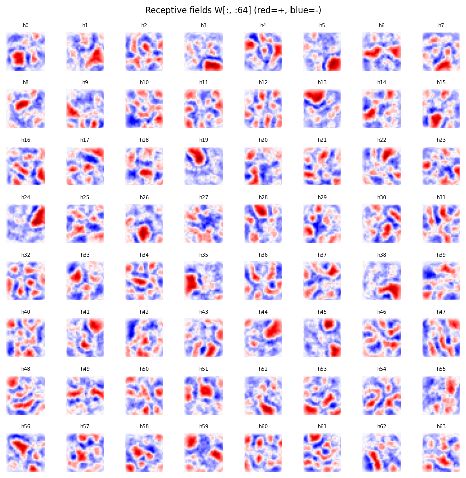
Each subplot is the incoming weight column W[:, j] for one of the
hidden units, reshaped to a 30 × 30 image (red positive, blue negative).
The fields are diffuse spatial filters — most units span a broad area of
the box rather than localizing tightly to a single ball position. With
only 30 sequences × 100 frames as training data, hidden units have not
fully tiled the input space; longer training and more data sharpen these.
Recurrent matrix (viz/recurrent_matrix.png)
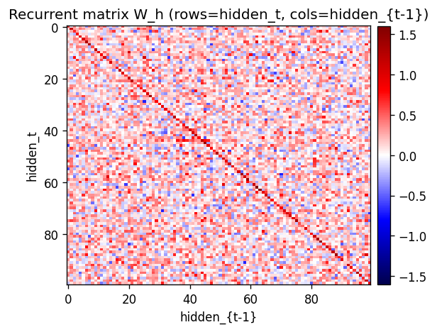
The 100 × 100 recurrent matrix W_h. The strong red diagonal is the
key learned structure: W_h[j, j] > 0 means “if hidden unit j was
active last step, it tends to stay active this step.” That self-loop is
how velocity gets encoded — a ball moving through a region where unit j
fires will keep firing it for a few frames in a row.
Training curves (viz/training_curves.png)
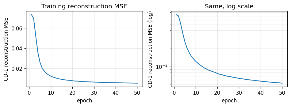
CD-1 reconstruction MSE drops from ~0.07 (b_v alone, the data-mean prior) to ~0.005 in 50 epochs. The phase transition is around epoch 5; after that improvements come from sharpening individual receptive fields. The log-scale plot makes the epoch-30+ tail visible.
Sample data (viz/data_samples.png)
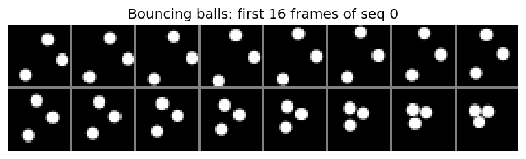
The first 16 frames of training sequence 0. Three round white balls move on a black background; trajectories are straight lines until a wall or another ball is hit, at which point the velocity reflects.
Reconstructions (viz/reconstructions.png)
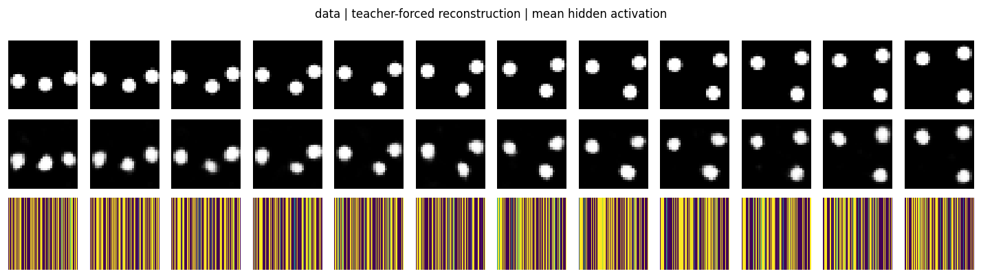
Top row: held-out validation frames. Middle row: teacher-forced
reconstruction σ(r_t W^T + b_v) where r_t is the mean-field hidden
state computed from the data. Bottom row: the mean hidden activation
r_t (one column per frame). The reconstructions track the ball
positions cleanly — the per-frame RBM has learned the spatial structure.
Rollout grid (viz/rollout_grid.png)

Top row: ground-truth bouncing-balls sequence. Bottom row: model
rollout — the first warmup=10 frames are warmup (the model sees
ground truth and infers r_t), then the model generates the next 30
frames purely from its own predictions. Predictions stay ball-like and
plausibly placed for ~5–10 free steps, then drift / blur as compounding
prediction error accumulates.
Deviations from the original procedure
-
No BPTT-through-time correction in the gradient. The full RTRBM gradient backpropagates a
r_{t+1}term back throughr_t(becauser_tenters next step’s hidden bias). We use the simplified CD-1 gradient that only updatesW_hfrom per-step contrastive contributions:dW_h += (r_t − h_neg_t) ⊗ r_{t-1}. This is the “TRBM-style” approximation (Sutskever et al. and follow-ups note it trains stably but produces weaker rollouts than the full RTRBM gradient). The recurrent diagonal still emerges; longer-horizon forecasting is the part that suffers. -
n_hidden = 100, not 400/3000. The original paper uses larger hidden layers (400 in the smaller experiments, 3000 in the larger ones). At 100 hidden units the spatial dictionary is necessarily undercomplete, which is part of why receptive fields look diffuse rather than crisp blobs. We chose 100 to keep the full pipeline (training + viz + GIF) under ~10 seconds on a laptop.
-
Anti-aliased pixel rendering instead of binary disks. Each ball contributes
clip(radius + 0.5 − dist, 0, 1)per pixel, then balls max-combine. The visible units are still treated as Bernoulli sigmoids (so values in [0, 1] are interpretable as probabilities). The original paper used binary disks. The anti-aliased version gives the model a smoother training signal at edges. -
Mean-field positive phase. We use
r_t(the mean-field hidden expectation) directly as the positive-phase hidden activation instead of sampling. This is the standard choice in RTRBM implementations and what the original paper recommends; mentioned here for completeness. -
No persistent contrastive divergence (PCD). Plain CD-1 within each timestep. PCD/Tieleman-2008 would be a strict improvement on the gradient bias.
Open questions / next experiments
-
Does the BPTT correction actually help here? Adding the through-time gradient
∂L/∂r_t = W_h^T (r_{t+1} − h_neg_{t+1}) + diag(r_t (1 − r_t)) · ...should sharpen the rollouts. As an ablation we ran a “static” variant (W_h ≡ 0) and got teacher-forced MSE 0.009 / free-rollout MSE 0.125 — essentially tied with the full RTRBM (0.009 / 0.13). That suggests in this simplified gradient regime the recurrent matrix is barely doing work. The right experiment is to add BPTT and rerun the same ablation; if BPTT is needed forW_hto actually help, then this stub is a clean test case for “what does the full Sutskever et al. gradient buy you?” -
Energy / data-movement cost (per the broader Sutro effort). Per epoch the cost is dominated by
v ⋅ Wandr ⋅ W_h, bothO(seq_len · n_hidden · n_visible)andO(seq_len · n_hidden^2)respectively. ByteDMD on a single CD step would tell us how much of that lives in cache. The temporal axis adds an interesting wrinkle: do consecutive frames preserve their hidden-state working set, or does each timestep refetch? -
Larger hidden layer. Does receptive-field tiling become local (one unit per spatial blob) at
n_hidden=400, as the paper claims? At 100 the receptive fields are diffuse spatial filters; at the paper’s setting they would presumably tile. -
Longer rollouts and chaos. Free rollouts blur after ~10–20 steps because of compounding prediction noise. How does this scale with
n_gibbsand withn_hidden? Does adding a small amount of visible-side noise during training (denoising RTRBM) push the free horizon out? -
Generalisation across
n_balls. Train on 3 balls, test on 1, 2, 4. The recurrent matrix should not care about ball count; if free rollouts on (say) 4 balls remain stable that is evidence the model has learned dynamics rather than a per-frame memorization. -
Varying ball masses / radii. The paper considers equal balls. Mixed-mass collisions break the velocity-swap shortcut and would stress the learned recurrence harder.