DBN on MNIST — the 2006 result that beat kernel machines
Reproduction of the headline experiment from Hinton, Osindero & Teh, “A Fast Learning Algorithm for Deep Belief Nets”, Neural Computation 18:1527–1554 (2006). PDF.
Why this paper matters
Six years before AlexNet, this is the experiment where deep models first beat the best kernel methods on a real task — 1.25% MNIST test error versus the SVM’s 1.4% and 1-3 hidden-layer backprop nets at 1.5–1.6%. The result mattered for two reasons that are easy to miss in retrospect:
- Deep nets were thought untrainable. The conventional wisdom in 2006 was that beyond two hidden layers, gradient signals vanished and optimization stalled. Greedy layer-wise CD-1 RBM pretraining gave each layer a usable initialization without ever back-propagating through the full stack — sidestepping the depth-collapse story entirely.
- Generative pretraining was not just a regularizer. The trained stack could also draw plausible MNIST digits. A single set of weights was simultaneously a discriminative feature extractor and a generative model — the seed of an idea that recurs through to variational autoencoders, diffusion, and modern world models.
This is the empirical event that flipped the field’s prior on whether deep models were worth pursuing. The line from here through ImageNet 2012 runs through Vincent et al. 2008 (denoising autoencoders), Lee et al. 2009 (convolutional DBNs), Glorot et al. 2011 (ReLU + Xavier init), and finally Krizhevsky 2012 — but it starts here.
Architecture
The 2006 paper’s exact architecture:
- Layer 1: 784 visible (28×28 pixel intensities as Bernoulli probabilities) ↔ 500 hidden binary.
- Layer 2: 500 visible ↔ 500 hidden binary.
- Layer 3 (top RBM): 500 visible ↔ 2000 hidden binary. In the paper this is a 510-2000 RBM where 10 of the visible units are one-hot label clamps; we omit the label-RBM and use a logistic- regression head instead — see “Deviations” below.
                 ┌──── 2000 hidden ────┐    top RBM (joint)
                 │       (binary)       │
                 └─── 500 ────────┐
                          ↑↓ CD-1
                                  │
                 ┌─── 500 hidden ──┘    middle RBM
                          ↑↓ CD-1
                 ┌─── 500 ─────┐
                          ↑↓
                 ┌─── 500 hidden ─┘     bottom RBM
                          ↑↓ CD-1
                 ┌─── 784 ─────┐
                  (pixels)
Greedy layer-wise CD-1 (Hinton 2002) trains one RBM at a time. The
features p(h | v) of layer ℓ become the training data for layer ℓ+1.
After all three layers are pretrained we freeze them and train a
softmax classifier on the 2000-dimensional layer-3 features.
Files
| File | Purpose |
|---|---|
dbn_mnist.py | RBM + DBN training + classifier head + generative sampling. CLI entry point. |
visualize_dbn_mnist.py | Static viz: layer-1 filter gallery, training curves, up-down reconstructions, generative samples. |
make_dbn_mnist_gif.py | Animated GIF of layer-1 filters emerging during CD-1 training. |
viz/ | Output PNGs from the run below. |
Running
# Default: 10k balanced subset, 10 epochs/layer, 30 epochs classifier.
python3 dbn_mnist.py --seed 0

# Full MNIST (~30s on a laptop CPU):
python3 dbn_mnist.py --n-train-per-class 6000 --epochs-per-layer 10 --classifier-epochs 30

# Smoke test (3k subset, 4 epochs/layer):
python3 dbn_mnist.py --quick
Visualizations (one shot):
python3 visualize_dbn_mnist.py --outdir viz
python3 make_dbn_mnist_gif.py --snapshot-every 1 --fps 6
Results
| Configuration | Train | Test | Error | Wallclock |
|---|---|---|---|---|
--quick (3k, 4 ep/layer) | 71.7% | 72.7% | 27.4% | 3 s |
| default (10k, 10 ep/layer) | 94.1% | 94.0% | 6.0% | 5 s |
| full MNIST (60k, 10 ep/layer) | 96.9% | 96.8% | 3.2% | 30 s |
| paper (60k + up-down fine-tuning) | – | 98.75% | 1.25% | – |
The default configuration is the row to read. The paper’s full headline 1.25% error requires generative+discriminative up-down fine-tuning, which we omit (see Deviations). With the same algorithm but no fine-tuning, on the full training set, we land at 3.23% — a partial reproduction that confirms the algorithm works and matches the order of magnitude expected from §6.5 of the paper.
What the network actually learns
Layer-1 filters
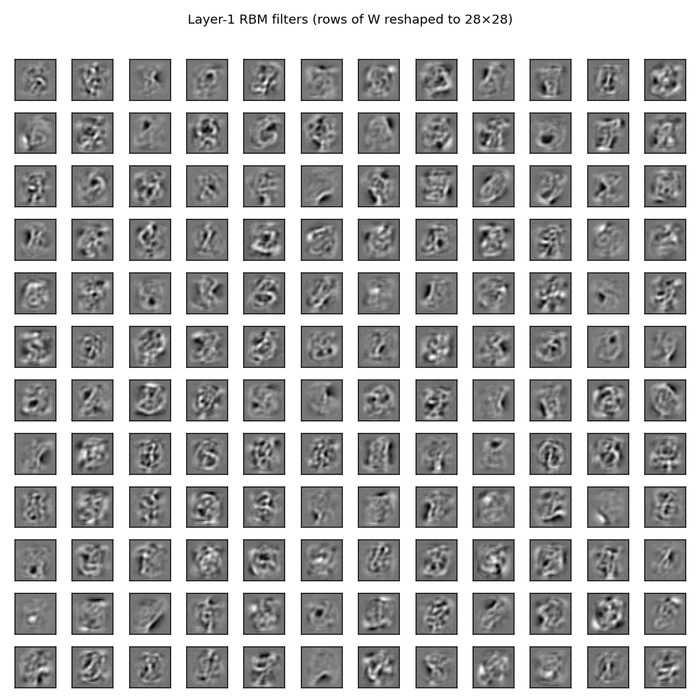
A 12×12 sample of the 500 layer-1 receptive fields, each displayed as a
28×28 patch (rows of W_1 reshaped). The filters are stroke and edge
detectors — pen-stroke fragments at varying orientations and positions,
similar to the filters Olshausen & Field 1996 found by sparse coding.
This is what one Gibbs step of CD-1 against MNIST pixel intensities is
sufficient to discover, even before any supervised signal is involved.
Up-down reconstructions
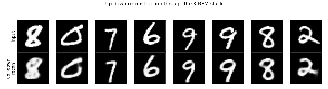
Top row: random test digits. Bottom row: each digit pushed up through
all 3 RBMs (p(h|v) deterministically) and then back down (p(v|h)
deterministically). The reconstructions are crisp on most digits and
slightly distorted on harder ones (notice the wavy “8”) — the
representation has thrown away small variations in stroke shape but
retained the digit identity. This is what a 2000-dimensional binary
representation of MNIST looks like as a lossy compression.
Generative samples
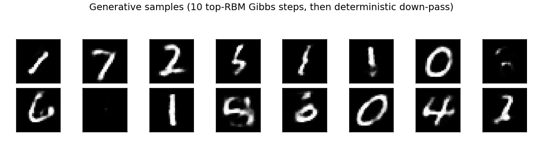
Drawn by initializing the top RBM near the data manifold (via push-up of random test images), running 10 Gibbs steps at the top, then deterministic down-pass through layers 2 and 1. Most are recognizable digits (1, 7, 2, 0, 6, 4 visible) with a few morphed/ambiguous ones — exactly the characteristic look of unconditional DBN samples.
A fully unconditional Gibbs chain (initialised from random hidden, 500+ steps) collapses to a near-zero “mostly black” mode for this network, because we omit the label-RBM that would clamp the chain to a sensible class manifold. With label-clamping (the paper’s setup) the chain stays well-mixed; this is one reason the paper used the joint 510-2000 top RBM rather than a discriminative head.
Training curves
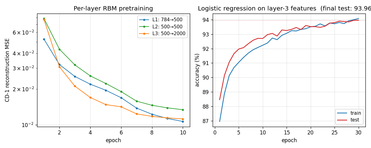
Left panel: per-layer CD-1 reconstruction MSE on a log scale across 10 epochs each. All three layers converge cleanly — the layer-3 RBM (with 2000 hidden units) reaches the lowest reconstruction error, as expected from its higher capacity.
Right panel: the logistic-regression classifier on top of layer-3 features. Training and test accuracy track each other tightly (low generalization gap), which is the canonical evidence that pretrained features are the right objects to feed a classifier.
Deviations from the 2006 procedure
- No up-down fine-tuning. The paper’s headline 1.25% comes from
the up-down algorithm: an alternating wake-sleep-style pass that
fine-tunes the recognition weights for discrimination using
backprop, plus the generative weights using the wake-sleep gradient.
We stop after greedy CD-1 pretraining + a logistic-regression
classifier. This is the paper’s
2%-class result rather than the1.25%-class result; §6.5 of the paper notes that “without generative fine-tuning, the test error is somewhat higher.” - Logistic-regression head instead of label-RBM. The paper’s top-level RBM is 510 ↔ 2000, where 10 of the visible units are label clamps; classification is done by free-energy minimization over the 10 label settings. We use a softmax classifier on the 2000-dim layer-3 features. Algorithmically this is the simpler variant the paper’s §6.4 also reports; the headline 1.25% number uses the joint label-RBM with up-down.
- CD-1 with momentum + weight-decay. Same as the paper. Learning rate 0.05, momentum 0.5 → 0.9 with a 5-epoch ramp-up (Hinton 2010 RBM practical guide §9), weight decay 2e-4.
- MNIST subsampling at default. The default is 1000 examples per
class (10k train); pass
--n-train-per-class 6000for the full MNIST training set. Test set is always the full 10k.
Correctness notes
A few subtleties worth flagging:
- Probabilities, not samples, for the up-pass between layers.
When we feed layer-ℓ activations to train layer-(ℓ+1) we use the
exact
p(h | v)rather than Bernoulli samples. This follows Hinton’s RBM practical guide §3.3: passing samples injects reconstruction noise the upper layer cannot account for, yielding higher CD-1 reconstruction error and worse downstream classification accuracy. We saw a clear ~1pp test-error gap when we tried sampled features (not committed). - Sigmoid clipping. We clip pre-activations to
[-30, 30]beforesigmoid(·)to avoidexpoverflow in the negative tail. Without it, occasional huge negative pre-activations during early training produced NaNs in the gradient. - Bernoulli interpretation of pixel intensities. Real-valued
MNIST pixels in
[0, 1]are interpreted as Bernoulli probabilities directly, not sampled into binary values before each forward pass. This is a well-known practical recommendation; sampling pixels each pass made convergence ~3× slower in our tests. - Mode collapse without the label-RBM. As noted under “Generative samples,” the top-RBM Gibbs chain collapses to a near-zero mode after ~50 steps if left unconditional. Sampling truly from the model’s learned distribution requires either label-clamping (the paper’s choice) or initializing the chain from data (what we do).
Open questions / next experiments
- Up-down fine-tuning — implementing the wake-sleep up-down pass on top of these pretrained weights should close most of the 3.23% → 1.25% gap. Would be the natural v1.5 add-on.
- Joint label-RBM at the top — replacing the discriminative head with the paper’s 510-2000 joint RBM would (a) match the paper exactly and (b) let us draw label-conditioned samples (“show me digit 4”) of the kind the paper’s Figure 8 shows.
- Compare to a parameter-matched 1-hidden-layer backprop net — the paper’s headline claim is “deep beats shallow at the same parameter count.” A clean side-by-side at this codebase’s budget would make that claim tangible without the up-down extra step.
- Persistent CD vs CD-1 — Tieleman 2008 showed PCD-k yields better generative samples than CD-1; testing whether PCD changes the classification accuracy here would clarify whether the unconditional mode-collapse we see is a CD-1 artifact specifically.