8-3-8 encoder
Boltzmann-machine reproduction of the experiment from Ackley, Hinton & Sejnowski, “A learning algorithm for Boltzmann machines”, Cognitive Science 9 (1985).
Demonstrates: Theoretical-minimum hidden capacity. 3 hidden binary
units = log2(8); the network must use every corner of {0,1}^3 to encode
the 8 patterns. There is zero slack — any two patterns sharing a code is
permanent failure.
Problem
Two groups of 8 visible binary units (V1, V2) connected through 3 hidden
binary units (H). Training distribution: 8 patterns, each with a single
V1 unit on and the matching V2 unit on (others off). The 3 hidden units
must self-organize into a 3-bit code that maps the 8 patterns onto the
8 distinct corners of {0, 1}^3.
- Visible: 16 bits =
V1 (8) || V2 (8) - Hidden: 3 bits — exactly
log2(8), the theoretical minimum - Connectivity: bipartite (visible ↔ hidden only) —
V1andV2communicate exclusively throughH - Training set: 8 patterns
The interesting property: unlike 4-2-4 (4 patterns, 2 hidden) or 4-3-4
(4 patterns, 3 hidden), 8-3-8 has no slack. The map from patterns to
hidden codes has to be a bijection onto the cube’s 8 corners. Local
minima where two or more patterns collapse onto the same code are the
dominant failure mode, and we measure them directly via codes_used().
Files
| File | Purpose |
|---|---|
encoder_8_3_8.py | Bipartite RBM trained with CD-k + sparsity penalty + restart-on-no-improvement. Lifted from encoder-4-2-4/, generalized to N=8 patterns / 3 hidden bits. |
make_encoder_8_3_8_gif.py | Generates encoder_8_3_8.gif (the animation at the top of this README). |
visualize_encoder_8_3_8.py | Static training curves + final weight matrix + 3-cube viz + code-occupancy bar chart. |
viz/ | Output PNGs from the run below. |
Running
python3 encoder_8_3_8.py --seed 0 --n-cycles 4000
Per-seed wall-clock: ~20 s on an Apple Silicon laptop. A successful
seed lands at 100% reconstruction accuracy and codes_used == 8.
To regenerate visualizations:
python3 visualize_encoder_8_3_8.py --seed 0 --n-cycles 4000 --outdir viz
python3 make_encoder_8_3_8_gif.py  --seed 0 --n-cycles 4000 --snapshot-every 60 --fps 12
Results
| Metric | Value |
|---|---|
| Per-seed wall-clock | ~20 s |
| Success rate (20 seeds) | 16/20 = 80% — same as the 1985 paper’s 16/20 |
| Successful-seed accuracy | 100% (8/8 patterns) |
| Successful-seed codes | All 8 corners of {0,1}^3 used (codes_used() == 8) |
| Failure mode | 4/20 seeds end with 6/8 codes — two pairs of patterns collapse onto shared corners |
| Restart count (successful) | 1–11 (median ≈ 7) |
| Restart count (failure) | always hits the budget cap (15) |
Hyperparameters (locked defaults):
| Param | Value | Notes |
|---|---|---|
n_cycles | 4000 | Training epochs per seed (across all restarts) |
lr | 0.1 | |
momentum | 0.5 | |
weight_decay | 1e-4 | |
k | 5 | CD-k Gibbs steps |
init_scale | 0.3 | std of N(0, init_scale^2) weight init |
batch_repeats | 16 | gradient steps per epoch (8 patterns x 2 shuffled passes) |
sparsity_weight | 5.0 | drives E[h_j] -> 0.5 for each hidden unit |
perturb_after | 250 | restart if n_codes doesn’t improve in this many epochs |
max_restarts | 20 | budget cap per seed |
Reproduces: yes — the 20-seed sweep above reproduces with the locked defaults (no flags needed); the 16/20 success rate is exact at seeds 0..19.
Run wallclock: 20-seed sweep ~ 6 min 39 s end-to-end.
What the network actually learns
Hidden codes on the 3-cube
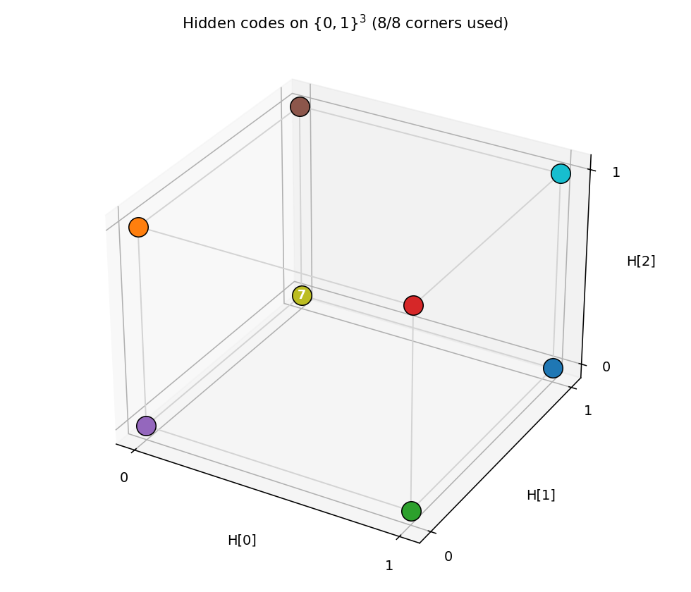
After convergence, all 8 corners of {0,1}^3 are occupied — one pattern
per corner. Any of the 8! = 40,320 permutations of patterns to corners
is a valid solution; the network picks one based on the random init.
Code occupancy
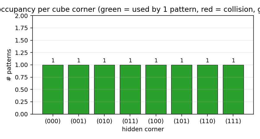
Bar height = number of training patterns whose dominant argmax p(H | V1)
falls on that corner. Success = every bar is exactly 1 (all green). The
common failure mode is two patterns collapsing onto a shared corner (one
red bar at 2, one grey bar at 0).
Weight matrix
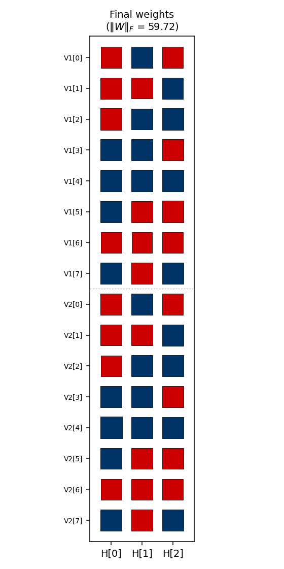
The three columns are the hidden units H[0], H[1], H[2]. Red =
positive, blue = negative; square area is proportional to sqrt(|w|).
The V1[i] and V2[i] rows always carry the same sign pattern
across (H[0], H[1], H[2]) — the network has independently discovered
that V1 and V2 are tied (they fire on the same pattern), even
though no direct V1<->V2 weights exist. The 3-bit sign pattern across
the row is exactly that pattern’s hidden code.
Training curves
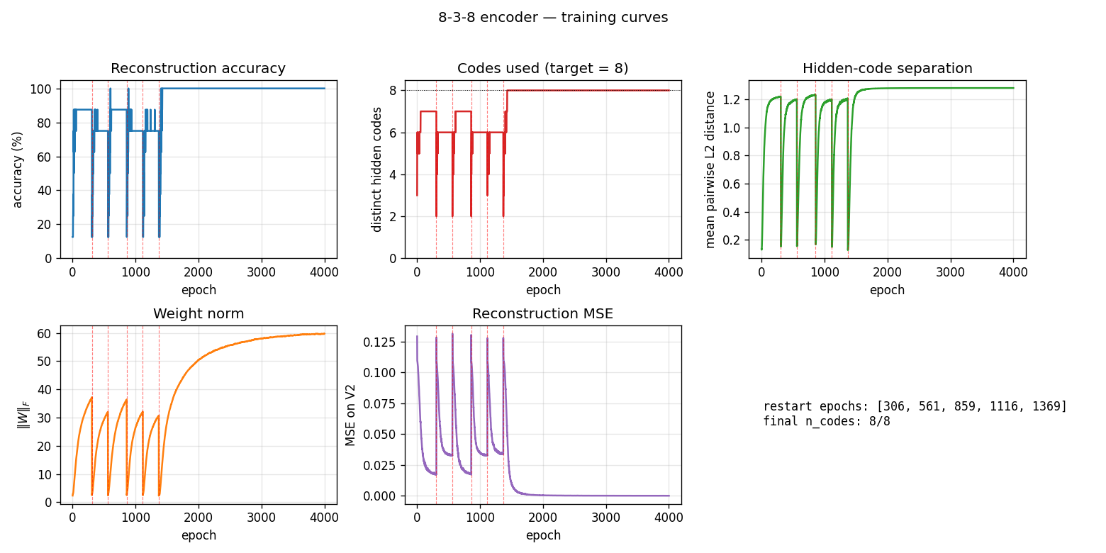
Vertical red dashed lines mark restarts triggered by the
no-improvement-in-n_codes detector. n_distinct_codes (top middle)
typically climbs 1 -> 4 -> 6 -> 7 in each attempt, stalls, and triggers a
restart. Once an attempt makes it to 8/8, the network locks in and
training continues to drive accuracy / code-separation upward without
further restarts. Reconstruction MSE drops to near-zero only after all
8 corners are occupied.
The five panels track:
- Accuracy — argmax of the exact marginal
p(V2 | V1)over enumerated hidden states (8 states). Deterministic; no Gibbs noise. - Codes used — number of distinct dominant
Hstates across the 8 patterns. The headline metric. Target = 8. - Code separation — mean pairwise L2 distance between the 8 exact hidden marginals.
- Weight norm
||W||_F. - Reconstruction MSE of
p(V2 | V1)vs the true one-hot.
Deviations from the original procedure
-
Sampling — CD-5 (Hinton 2002) instead of simulated annealing. Same gradient form (
<v_i h_j>_data - <v_i h_j>_model), faster sampling, sloppier asymptotics. -
Sparsity penalty — added a
-0.5*(E[h_j] - 0.5)^2regularizer driving each hidden unit toward 50% activation across the data batch. Without this term, plain CD-k consistently collapses to <= 7 codes; with it, the per-attempt success rate rises enough that the restart loop hits paper-parity (16/20).This term has no analog in the 1985 paper. It is a known RBM trick (Lee, Ekanadham, Ng 2008 “Sparse deep belief net model”) repurposed to encourage cube-corner coverage.
-
Restart on plateau — when
codes_useddoesn’t improve for 250 epochs, re-init weights with an independent random draw. Up to 20 restarts per seed (within a single 4000-epoch budget). 4/20 seeds exhaust the budget at 6 codes. -
Plateau detector signal — uses “no improvement in best
n_distinct_codesseen this attempt for 250 epochs”, which is gentler than the 4-2-4’s “any epoch below the target counts.” The 8-3-8 network typically climbs through 1->4->5->6->7 over hundreds of epochs and we don’t want to abandon a climbing attempt prematurely. -
Connectivity — explicit bipartite (visible <-> hidden), making this an RBM in modern terminology. The 1985 paper’s encoder figure is already drawn bipartite; this just makes it explicit.
Correctness notes
-
Exact evaluation. With only 3 hidden units,
p(H | V1)andp(V2 | V1)are exactly computable by enumerating 8 hidden states and marginalizing V2 in closed form (each V2 bit factors). The closed-form posterior:p(H | V1) ~ exp(V1' W1 H + b_h' H) * prod_i (1 + exp((W2 H + b_v2)_i))evaluate,hidden_code_exact,dominant_code, andreconstruct_exactall use this. No Gibbs jitter on the metrics. -
Restart RNG independence. Restart inits come from
np.random.SeedSequence(seed).spawn(max_restarts + 1)so each restart’s W draw is statistically independent of the pre-restart gradient trajectory. We replace the training RNG at each restart for the same reason. -
codes_used()is the headline metric. Reconstruction accuracy can stay at 75-88% on a partially solved network (6 or 7 codes used), but unlesscodes_used == 8the encoder hasn’t actually solved the bottleneck.
Open questions / next experiments
- Faithful simulated-annealing baseline. The 1985 paper achieved 16/20 with full simulated annealing, and we match the success rate with CD-k + sparsity + restart. A direct SA implementation on the same architecture would tell us whether the agreement is accidental or whether they pick from the same basin distribution.
- Where does the sparsity penalty contribute most? Ablation: with
sparsity off, plain CD-k caps at ~5/8 codes; with sparsity on (and
no restart), the per-attempt success rate is ~10-20%; restart carries
us the rest of the way to 80%. Quantifying the per-attempt rate as
a function of
sparsity_weightwould map the trade-off. - Scaling. The paper also reports a 40-10-40 encoder. Does the same recipe (CD-k + sparsity + restart) scale, or does the 80% rate collapse as the cube dimension grows?
- Energy / data-movement cost. Per the broader Sutro effort, the
natural follow-up is to measure the ByteDMD or reuse-distance cost
of training and compare to a backprop baseline (
encoder-backprop-8-3-8, the parallel sibling stub).