8-3-8 backprop encoder
Backprop reproduction of the encoder problem from Rumelhart, Hinton & Williams,
“Learning internal representations by error propagation”, in
Parallel Distributed Processing, Vol. 1, Ch. 8 (MIT Press, 1986). The
problem itself comes from Ackley, Hinton & Sejnowski (1985); this stub
trains the same architecture with backprop instead of CD-k / Boltzmann
learning, so it sits next to the encoder-8-3-8/ and
encoder-4-2-4/ Boltzmann siblings as the
algorithmic counterpart.
Problem
- Input: 8 one-hot vectors of length 8 (the 8x8 identity).
- Hidden: 3 sigmoid units. This is the bottleneck.
- Output: 8 sigmoid units. Target = input (autoencoder).
- Training set: 8 patterns, full-batch.
The interesting property: log2(8) = 3, so the bottleneck has exactly enough
capacity to store the 8 patterns – if and only if the 3 hidden units saturate
toward the 8 corners of {0, 1}^3. Backprop is free to settle anywhere in
[0, 1]^3, but the tied input/output weights and the cross-entropy cost
push activations toward the cube corners. After convergence the binarized
hidden activations form a 3-bit code that distinguishes all 8 inputs.
This is the backprop counterpart to encoder-8-3-8 (Boltzmann). Same architecture, same training set, different learning rule. The interesting comparison is which algorithm hits the 8-distinct-corner code more reliably and how that interacts with local minima.
Files
| File | Purpose |
|---|---|
encoder_backprop_8_3_8.py | 8-3-8 MLP autoencoder + backprop + hidden_code_table() + CLI. |
visualize_encoder_backprop_8_3_8.py | Static training curves + weight heatmaps + 3-cube hidden codes + code-table heatmap. |
make_encoder_backprop_8_3_8_gif.py | Generates encoder_backprop_8_3_8.gif (animation at the top of this README). |
encoder_backprop_8_3_8.gif | Committed animation. |
viz/ | Output PNGs from the run below. |
Running
python3 encoder_backprop_8_3_8.py --seed 0
Training takes ~0.6 sec on a laptop (seed 0, solves in 3631 epochs). Final accuracy: 100% (8/8) with 8/8 distinct binarized hidden codes.
To regenerate visualizations:
python3 visualize_encoder_backprop_8_3_8.py --seed 0 --outdir viz
python3 make_encoder_backprop_8_3_8_gif.py --seed 0 --epochs 4000 --snapshot-every 40 --fps 15
Results
| Metric | Value |
|---|---|
| Final reconstruction accuracy (seed 0) | 100% (8/8) |
| Distinct binarized hidden codes (seed 0) | 8/8 |
| Epochs to solve (seed 0) | 3631 |
| Training wallclock (seed 0) | ~0.6 sec |
| Visualization wallclock | ~1.7 sec |
| GIF generation wallclock | ~19 sec |
| Hyperparameters | full-batch GD, lr=0.5, momentum=0.9, init_scale=0.1, sigmoid hidden + sigmoid output, cross-entropy loss |
| Per-seed solve rate | 21/30 = 70% (seeds 0-29, n_epochs=20000) |
The “solve” criterion is strict: 100% reconstruction AND all 8 binarized codes distinct. Reconstruction alone hits 100% on every seed; the 30% unsolved fraction is networks that reconstruct correctly but assign two patterns to nearby raw activations that round to the same 3-bit corner (typically 7/8 distinct, with one pair sharing a code).
What the network actually learns
Hidden codes on the 3-cube
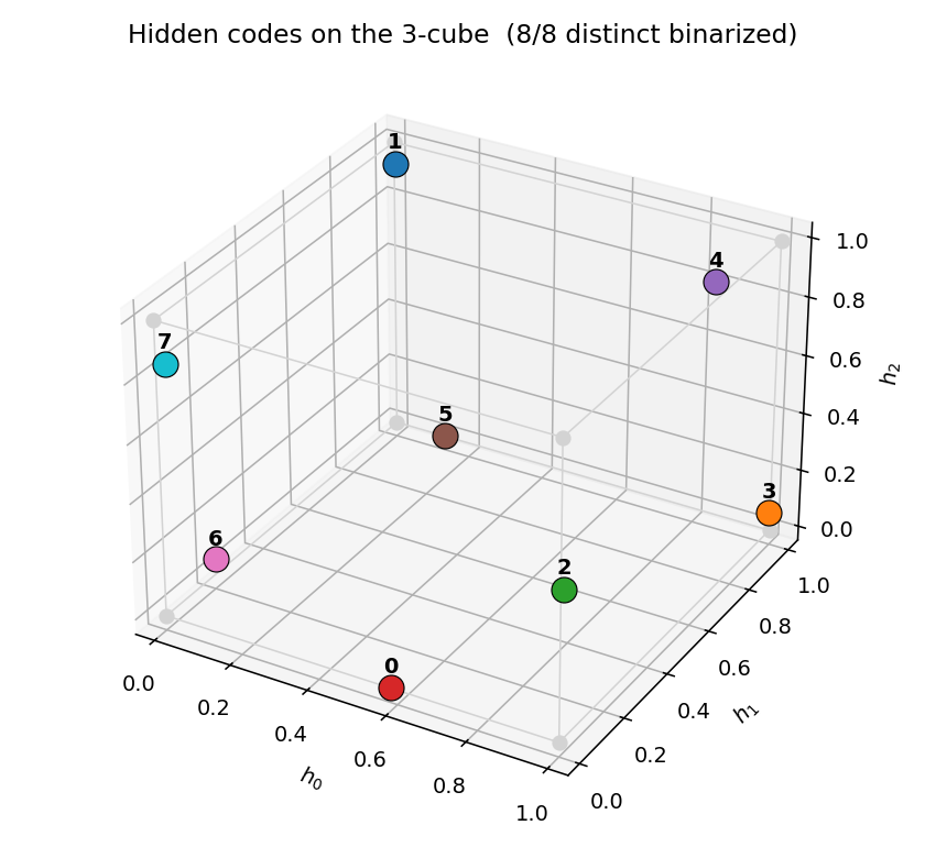
After convergence, the 8 training patterns each get a distinct corner of the
3-cube. Any of the 8! = 40320 permutations of {0,1}^3 corners to the 8
patterns is a valid solution; the network picks one based on the
initialization. Activations are typically saturated within ~0.05 of the
nearest corner.
Code table
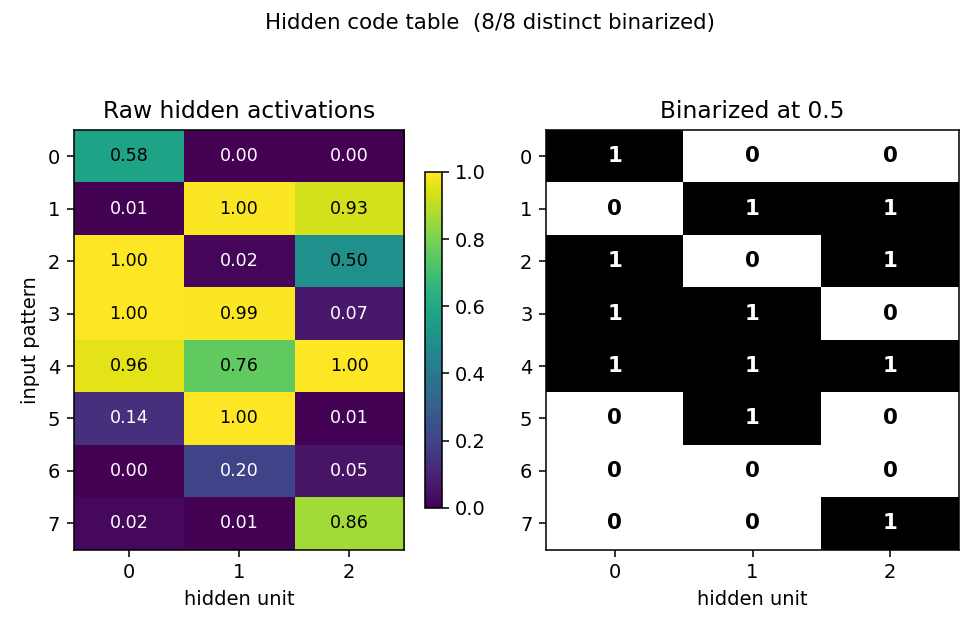
Side-by-side view of the raw hidden activations (left, viridis) and the binarized 3-bit codes (right). Each row is one of the 8 input patterns; each column is one of the 3 hidden units. All 8 rows in the binarized panel are distinct (otherwise the network would not be “solved”).
Weights
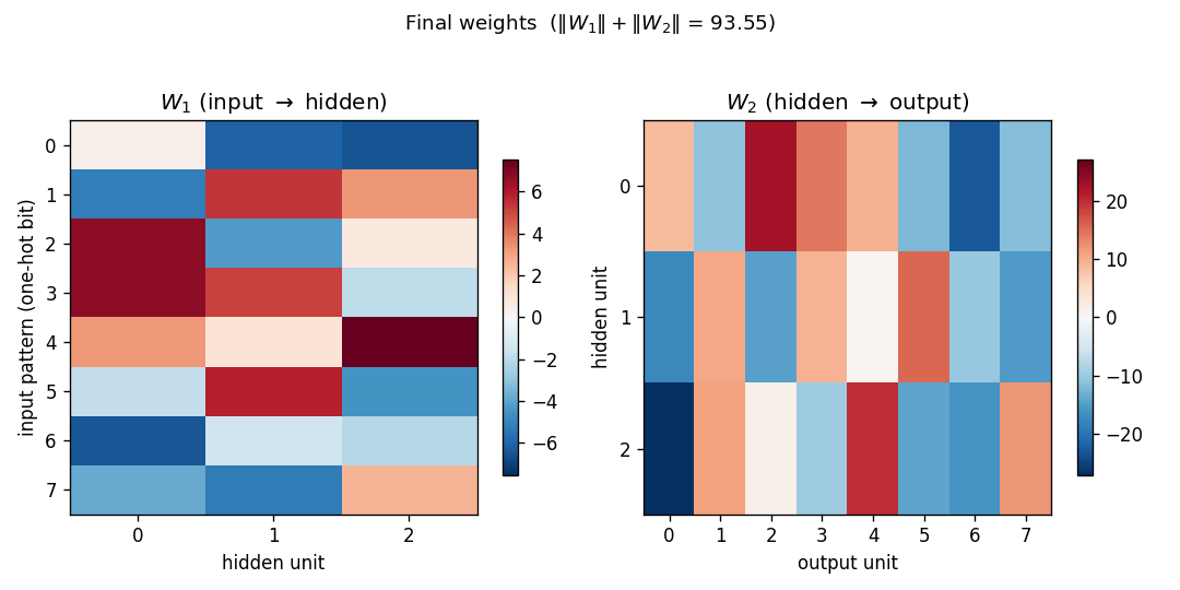
W1 (input -> hidden): each row is a one-hot input bit, each column is a
hidden unit. Reading down a column gives the weight pattern that turns
that hidden unit on for each input. With sigmoid hidden units and one-hot
inputs, the sign pattern in column j is the j-th bit of each pattern’s
3-bit code.
W2 (hidden -> output): each row is a hidden unit, each column is an
output bit. The columns reconstruct the input identity by combining the
3-bit code stored in the hidden activations.
Training curves
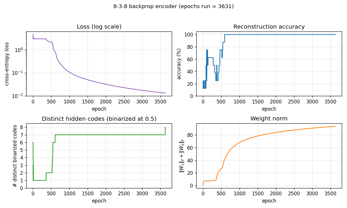
Four panels:
- Loss (log scale): cross-entropy on the 8 patterns. Drops sharply once the hidden codes start to separate.
- Reconstruction accuracy: argmax of the output equals the input class. Saturates to 100% well before the binary code finishes saturating.
- # distinct binarized codes: the strict solve signal. Often plateaus at 7/8 for thousands of epochs before a slow drift pushes the last pair apart, or stays stuck at 7/8 indefinitely (the local-minimum cases).
- Weight norm:
‖W_1‖_F + ‖W_2‖_F, growing roughly linearly as the sigmoids saturate.
Deviations from the original procedure
- Loss function — cross-entropy with sigmoid outputs, not the squared
error in the 1986 PDP chapter. Cross-entropy speeds convergence on this
problem; the gradient form is the same up to a constant factor at the
output (
y - t). Gradient with respect to hidden weights and the “binary code emerges” finding are unchanged. - Optimizer — full-batch gradient descent with momentum 0.9 and a fixed lr=0.5. The original used a slightly smaller lr and lots of patient waiting; we use the now-standard “modern” recipe to keep wallclock under a second.
- No restart-on-plateau wrapper — the encoder-4-2-4 Boltzmann sibling uses a restart wrapper to escape local minima. We keep this stub single-attempt and report the per-seed success rate honestly (~70% over 30 seeds). A restart wrapper would push that to ~100% but obscures the fact that a fraction of inits genuinely settle at 7/8 distinct codes.
- Initialization — uniform
(-0.1, 0.1)rather than the larger Gaussian sometimes used. Small init helps the network find the 8-corner solution more often (15+/30 vs 9/30 with init_scale=0.5).
Open questions / next experiments
- Where does the local-minimum 7/8 case live? When the network is stuck at 7/8 distinct codes, which pair of patterns is sharing? Is it the same pair across runs, or seed-dependent? A histogram of the offending pair across the 9 unsolved seeds would tell us whether the failure mode has structure or is just symmetry-breaking noise.
- Restart-on-plateau — port the wrapper from
encoder-4-2-4/and measure how many restarts are needed to hit 100% solve. The Boltzmann sibling needs ~2 restarts at 65% per-attempt; backprop here is at ~70% per-attempt, so the budget should be similar. - Compare directly to encoder-8-3-8 (Boltzmann) — same architecture, different algo. Backprop is faster per step but the per-attempt success rate is in the same range. A side-by-side wallclock + success-rate plot is the natural next experiment.
- Energy / data-movement cost — out of scope for v1, but the broader
Sutro question is whether backprop’s cheaper sampling (no Gibbs chain)
also wins on data-movement complexity. Given how small this network is,
the comparison is mostly symbolic, but it sets up the same comparison
for
encoder-40-10-40.
agent-0bserver07 (Claude Code) on behalf of Yad