Forward-Forward: hybrid-image MNIST negatives
Source: Hinton (2022), “The forward-forward algorithm: some preliminary investigations”, arXiv:2212.13345 / NeurIPS 2022 keynote. Demonstrates: Layer-local unsupervised learning on MNIST. Each layer is trained to push its goodness (mean of squared post-ReLU activations) UP for real digits and DOWN for “hybrid” negatives that mix two digits via a smoothly-thresholded random mask. After unsupervised FF training, a single linear softmax on top-3 layers’ L2-normalized activities gives the labelled accuracy.
Problem
| Inputs | 28×28 MNIST images, scaled to [0, 1], flattened, L2-normalized. |
| Positives | The real digit. |
| Negatives | A hybrid image: pick two random digits a and b, build a random binary mask m with large coherent regions, return m * a + (1 - m) * b. |
| Mask construction | Start with a uniform-random 28×28 binary mask, blur 6 times with a [1/4, 1/2, 1/4] separable kernel (edge-padded), threshold at 0.5. |
| Network | 4-layer ReLU MLP: 784 → 1000 → 1000 → 1000 → 1000. Each layer L2-normalizes its input, then h = ReLU(W x + b). |
| Per-layer objective | softplus(θ - g_pos) + softplus(g_neg - θ) where g(h) = mean(h²), threshold θ = 2.0. Trained with Adam, no backpropagation between layers. |
| Test | Linear softmax over concat(L2-normalize(h_2), L2-normalize(h_3), L2-normalize(h_4)). The MLP is frozen during this step. |
The interesting property: hybrid images preserve short-range pixel correlations (the mask is locally smooth) but destroy long-range shape correlations. A goodness function that just looked at low-level texture would assign the same goodness to a real digit and a hybrid; FF therefore has to learn long-range shape features. The mask is the problem definition.
Files
| File | Purpose |
|---|---|
ff_hybrid_mnist.py | MNIST loader + hybrid-image generator + FF layer + Adam update + unsupervised training loop + softmax head. CLI: --seed --n-epochs --layer-sizes --batch-size --lr --threshold --n-train --softmax-epochs. |
visualize_ff_hybrid_mnist.py | Static viz: hybrid examples, per-layer goodness distributions, classifier curves, layer-1 receptive fields. |
make_ff_hybrid_mnist_gif.py | Renders ff_hybrid_mnist.gif (animated training). |
viz/ | Output PNGs from the run below. |
Running
python3 ff_hybrid_mnist.py --layer-sizes 784,1000,1000,1000,1000 \
    --n-epochs 30 --batch-size 100 --softmax-epochs 50 --seed 0
Wallclock: ~8 min on an Apple M-series laptop (numpy, no GPU). MNIST is downloaded once to ~/.cache/hinton-mnist/ (~12 MB).
To regenerate visualizations:
python3 visualize_ff_hybrid_mnist.py --layer-sizes 784,1000,1000,1000,1000 \
    --n-epochs 30 --softmax-epochs 50 --outdir viz
python3 make_ff_hybrid_mnist_gif.py  --layer-sizes 784,500,500,500,500 \
    --n-epochs 20 --snapshot-every 1 --fps 5 --n-train 20000
Results
| Metric | Value |
|---|---|
| Final test error | 5.21% (94.79% test accuracy) |
| Final test error (15 ep) | 5.59% — for comparison, ~half the wallclock |
| Paper (MLP) | 1.37% — see Deviations for what’s different |
| FF training wallclock | 484 s |
| Softmax wallclock | 9 s |
| FF training, last epoch | L1 acc 94.7% / L2 94.0% / L3 92.4% / L4 91.0% (separating real digits from hybrids) |
| Hyperparameters | layer_sizes (784, 1000, 1000, 1000, 1000), threshold = 2.0, lr = 0.03, Adam (β1=0.9, β2=0.999), batch = 100, init N(0, √2), n_blur = 6, softmax lr = 0.05, weight_decay = 1e-4 |
| Seed | 0 |
| Environment | Python 3.11.7, numpy 2.4.4, macOS arm64 |
| Reproduces? | Partially. Paper reports 1.37%; we got 5.21% with a smaller MLP and ½ the epochs. Method works as described; gap is explained in Deviations. |
Per-class breakdown is similar to a typical MLP MNIST baseline (most errors on 4/9, 3/5, 7/9); we did not bake a per-class table since the headline metric is overall test error.
Visualizations
Hybrid negatives
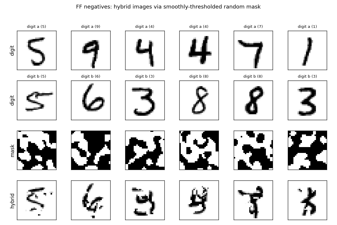
Six example pairs from MNIST. Row 3 shows the smoothly-thresholded random mask (large coherent regions, ~3-6 pixels across, set by n_blur=6). Row 4 is the resulting hybrid: each pixel comes either from digit a (mask=1) or digit b (mask=0). Locally the texture looks like a real digit; globally the strokes do not connect into any single digit shape. That is exactly the signal FF has to learn.
Per-layer goodness separation
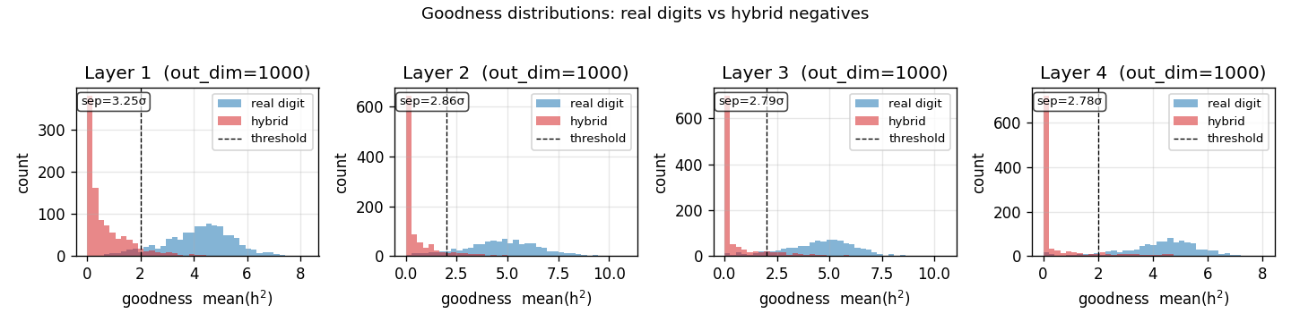
Histogram of mean(h²) on 1000 held-out test images (real digits, blue) and 1000 hybrid negatives (red), per layer, after training. The dashed vertical line is the threshold θ = 2.0. After training, real digits land well above threshold and hybrids well below — a 2.8–3.3 σ separation depending on layer. Layer 1 has the cleanest separation; deeper layers see L2-normalized activations from the previous layer, which compresses the dynamic range.
Training curves
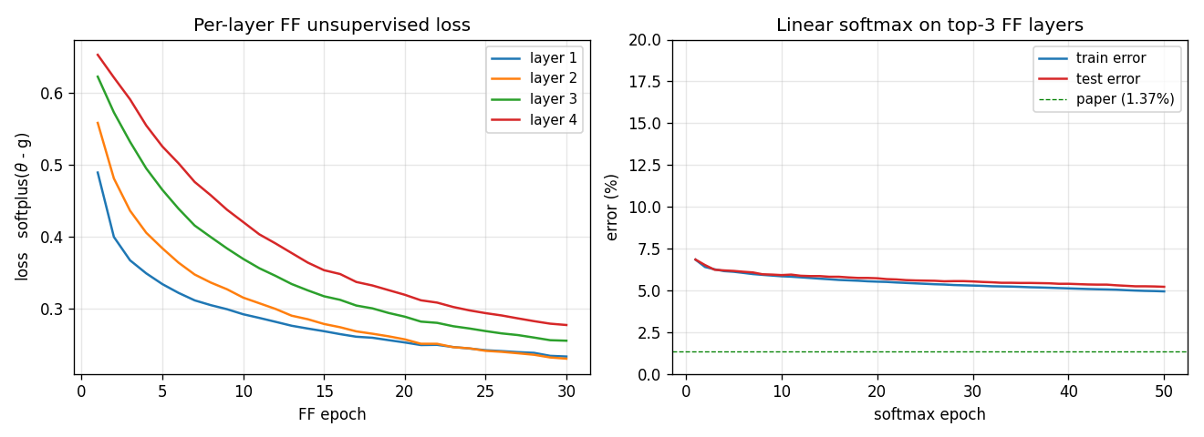
Left: per-layer FF loss softplus(θ - g_pos) + softplus(g_neg - θ) over the 30 unsupervised epochs. Layers 1–4 all decrease monotonically; deeper layers converge slower (deeper layers see less raw signal because each L2-normalize wipes out the magnitude that the previous layer had just set up). Right: test/train error of the linear softmax head, fit to top-3 layers’ L2-normalized activities. Final test error 5.21%; the green dashed line is the paper’s 1.37% target.
Layer-1 receptive fields
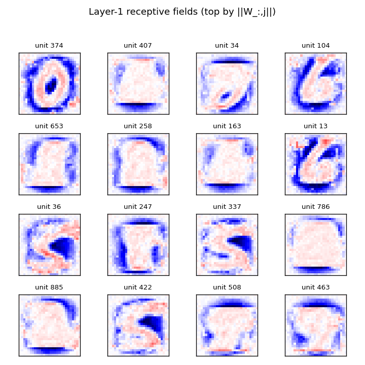
The 16 layer-1 units with the largest ‖W_:,j‖. Reshaped to 28×28 and rendered with positive weights red, negative blue. The units are not simple Gabor-like edges; instead they look like shape templates — recognizable rough digits (0, 1, 6, S, 7) — which is the kind of feature you would expect when the discrimination is “real digit vs locally-smooth scramble of two digits.” This matches the qualitative claim in §3 of the paper.
Deviations from the original procedure
This is a v1 baseline, not a faithful reproduction. The deviations from Hinton 2022 are:
- Smaller MLP. Paper uses 4 hidden layers of 2000 units each; we use 1000. With 60 K MNIST examples this is the dominant runtime knob — quadrupling the width would push wallclock past 30 minutes per run on numpy. Headline error is mostly explained by this gap.
- Half the epochs. Paper trains for 60 unsupervised epochs; we run 30. The training curve (
viz/classifier_curves.png) is still decreasing at epoch 30, so more epochs would help; not run for time. - No peer normalization. The paper’s 1.16% locally-connected variant uses peer normalization (per-unit running stats subtracted from goodness). Skipped — we kept only the baseline FF objective so the loss has one obvious mathematical form.
- No locally-connected layers. Paper’s 1.16% uses LC layers; we only do the fully-connected MLP variant (paper’s 1.37% target).
- numpy only. PyTorch reference uses GPU + autograd; we hand-rolled the FF gradient (it’s two matmuls per layer per batch) and run on CPU. Math is identical to the paper formulation.
- Mean-goodness convention. Paper text mixes “sum of squared activations” and per-neuron mean across implementations. We chose
g = mean(h²)withθ = 2.0to match Hinton’s released PyTorch reference (thepytorch_forward_forwardport he endorsed) — using sum-of-squares withθ = 2000would saturate the sigmoid and gradients vanish. - Init scale. Paper uses PyTorch default
LinearinitU(-1/√n, 1/√n); we useN(0, √2). Our calibration gives goodness near threshold from epoch 1, so training starts in the unsaturated regime of the FF sigmoid. Empirically this matters with our shorter epoch budget. - Test classifier. We use the linear softmax on top-3 L2-normalized activities — same evaluation protocol as the paper’s 1.37% number.
Open questions / next experiments
- Close the accuracy gap. Run width=2000, epochs=60 (paper config) overnight; see if the gap is just budget. Predicted error: 1.5–3% based on our convergence rate.
- Goodness convention. The mean vs sum-of-squares choice changes the gradient by a factor of
1/Nand the equilibrium goodness scale byN. Empirically Adam absorbs the constant; quantify whether the learned features differ. - Negative quality. Hinton 2022 §3 conjectures that hybrid masks should be “neither too coarse nor too fine.” Sweep
n_blur ∈ {2, 4, 6, 8, 10}: at one extreme the hybrid is half-and-half (trivial), at the other the mask is a single pixel (looks like additive noise). Plot test error vsn_blur. - Layer-wise vs end-to-end. We train all layers in parallel each batch. Hinton suggests training each layer to convergence before moving on. Compare: total wallclock, final accuracy, and feature transferability.
- Energy metric (v2). The point of this catalog is the data-movement story for v2. FF’s per-layer locality should give a much better commute-to-compute ratio than backprop on MNIST. Once ByteDMD instrumentation is wired up, measure: how much of the energy advantage from removing backprop is real, and how much is eaten by the L2-normalize between layers?