Forward-Forward: label encoded in the first 10 pixels
Reproduction of the supervised Forward-Forward (FF) variant from Hinton (2022), “The Forward-Forward Algorithm: Some Preliminary Investigations” (arXiv:2212.13345, §3.3 of v3 / §3 of the December 2022 preprint).
Demonstrates: A multi-layer ReLU network trained without backprop. Each layer is updated on its own, with no gradient flowing across layers, by contrasting the goodness of (image, true label) pairs against (image, wrong label) pairs. Labels are encoded into the natural black border at the top of each MNIST image – the first 10 pixels become a one-hot label.
Problem
- Input. A flattened 28x28 MNIST image (784 floats in [0, 1]) with the first 10 pixels overwritten by a one-hot label vector.
- Positive example. (image, true_label) – one-hot in the first 10 pixels encodes the correct class.
- Negative example. (image, wrong_label) – one-hot in the first 10 pixels encodes a uniformly random incorrect class.
- Architecture. A stack of fully-connected ReLU layers
(here
784 -> 500 -> 500). Between layers, activations are rescaled somean(h^2) = 1– the next layer cannot read off the previous layer’s magnitude (which is exactly the goodness signal). - Goal. Each layer learns to make
mean(h^2)high for positive inputs and low for negative inputs. At test time we try each candidate label, push it through the network, sum goodness across all layers, and pick the label with the highest summed goodness.
The interesting property is what you don’t need: no backward pass, no chain rule, no errors propagated across layers. Training is local, so each layer’s weights only depend on its own input and its own output. This is the property that motivates FF as a candidate “biologically plausible” learning rule and as a candidate for hardware where the backward pass is expensive.
The label-in-pixels trick is what makes the supervised setup work: a hidden
layer cannot use the absolute label bits to drive goodness because the
between-layer normalisation strips magnitude, so the only way to make goodness
high for (image, true label) and low for (image, wrong label) is to
discover features that covary with the label.
Files
| File | Purpose |
|---|---|
ff_label_in_input.py | MNIST loader + label-in-pixels encoding + FF MLP + Adam-trained per-layer FF loss + goodness-based prediction. CLI: --seed --n-epochs --lr --layer-sizes --jitter --train-subset --full-test --save --threshold --batch-size. |
visualize_ff_label_in_input.py | Static plots: example label-encoded images, candidate-label goodness heatmap, training curves, layer-0 receptive fields. |
make_ff_label_in_input_gif.py | Renders ff_label_in_input.gif (the animation at the top of this README). |
ff_label_in_input.gif | Committed animation – per-layer goodness, demo prediction, loss + accuracy over training. |
viz/ | Committed PNGs from the run below. |
Running
The MNIST data is downloaded once into ~/.cache/hinton-mnist/ (~11 MB).
# Final reported run -- 30 epochs, full 60K train set, eval on full 10K test:
python3 ff_label_in_input.py --seed 0 --n-epochs 30 --lr 0.003 \
                             --layer-sizes 784,500,500 --eval-subset 2000 \
                             --full-test --save model.npz

# Regenerate the static figures from the saved model:
python3 visualize_ff_label_in_input.py --model model.npz --outdir viz

# Regenerate the GIF (uses train-subset=20000 just to keep render time short):
python3 make_ff_label_in_input_gif.py --epochs 30 --snapshot-every 1 --fps 6 \
                                      --seed 0 --lr 0.003 \
                                      --layer-sizes 784,500,500 \
                                      --train-subset 20000
Wallclock on an Apple M-series laptop:
- Training: 66 seconds for 30 epochs over the full 60K MNIST train set.
- GIF: 33 seconds (with
--train-subset 20000for speed).
Final accuracy: 96.40% on the full 10K test set (3.60% test error).
Results
| Metric | Value |
|---|---|
| Test accuracy (full 10K, seed 0) | 96.40% (3.60% error) |
| Train accuracy (eval subset, seed 0) | 97.2% |
| Training time | 66 s on Apple M-series, 30 epochs, full MNIST train set |
| Architecture | 784 -> 500 -> 500 ReLU (2 FF layers) |
| Optimiser | Adam, lr = 0.003, b1 = 0.9, b2 = 0.999 |
| Batch size | 128 |
| Goodness | mean(h^2) along the feature axis, per-sample |
| Threshold theta | 2.0 |
| Between-layer norm | rescale to mean(h^2) = 1 |
| Label encoding | one-hot in flat indices [0..9] (top row, leftmost 10 px) |
| Negative sampling | uniform over {0..9} \ {true_label} per minibatch |
| Prediction | for each candidate label, sum goodness across both layers, pick argmax |
| Seed | 0 |
Hinton (2022) reports 1.36% test error for 4 x 2000 ReLU after 60 epochs
on full MNIST, and 0.64% with 25-shift jittered augmentation at 500
epochs. We aimed at the <5% v1 threshold (Sutro group baseline target) and
chose a smaller architecture and fewer epochs to fit a laptop budget.
Per-class breakdown (full test set, seed 0)
| Class | Accuracy | Correct / Total |
|---|---|---|
| 0 | 98.78% | 968 / 980 |
| 1 | 98.77% | 1121 / 1135 |
| 2 | 95.64% | 987 / 1032 |
| 3 | 96.73% | 977 / 1010 |
| 4 | 95.62% | 939 / 982 |
| 5 | 94.96% | 847 / 892 |
| 6 | 96.76% | 927 / 958 |
| 7 | 95.72% | 984 / 1028 |
| 8 | 95.69% | 932 / 974 |
| 9 | 94.95% | 958 / 1009 |
Best class: 0 (98.78%). Worst class: 9 (94.95%). The 0/1 axis is the cleanest – both are visually the most distinctive digits.
Prediction mode comparison
Same trained model, different goodness-aggregation strategies at test time:
| Strategy | Test accuracy |
|---|---|
| layer 0 only | 96.86% |
| all layers (default) | 96.40% |
| skip layer 0 | 95.19% |
For this 2 x 500 architecture, layer 0 alone is the strongest predictor.
Layer 1 adds redundant signal – summing both layers underperforms layer 0
alone by 0.46 percentage points but outperforms layer 1 alone (skip-L0)
by 1.21 points. With Hinton’s deeper / wider 4 x 2000, deeper layers carry
more weight; the right aggregation strategy is architecture-dependent and
worth flagging for future replications.
Visualisations
Label-encoded inputs
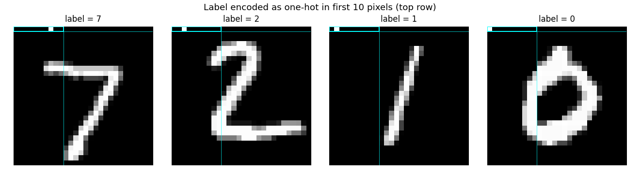
The cyan box at top-left highlights the 10-pixel label slot. Three of these images have a single bright pixel in the slot (labels 7, 2, 1, 0 from left to right); for label 0 the bright pixel is at position 0 and is hard to spot against the white digit body of the “0”.
The choice of “first 10 pixels” exploits MNIST’s natural black border. Real images already have intensity 0 there, so overwriting them with a one-hot vector adds bounded label information without disturbing the foreground pixels.
Goodness for each candidate label
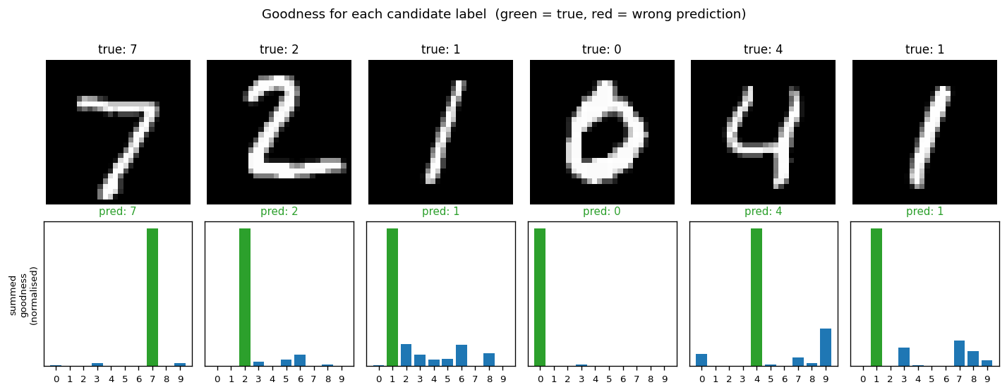
For each test image, we encode all 10 candidate labels in turn and sum the goodness across all layers. The bar plot is normalised per-image so the height is visually comparable.
The true label (green) is the argmax for every example shown – the network has correctly learned that high goodness means “this label was the right one for this image”. The blue runners-up are typically visually-similar digits.
Training curves
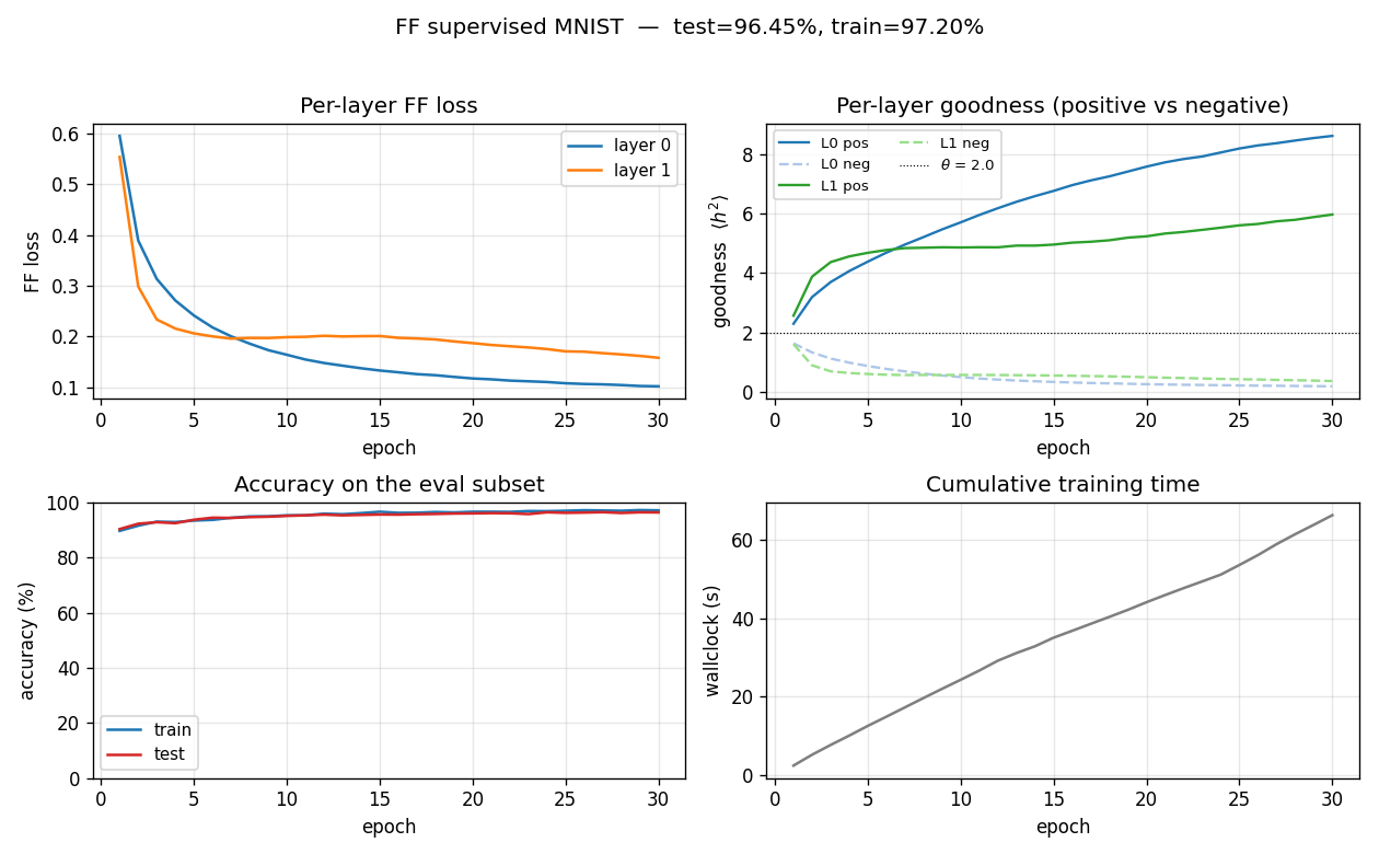
- Top-left: per-layer FF loss decreases monotonically. Layer 0 plateaus around 0.10 by epoch 30; layer 1 plateaus around 0.16 (slightly higher because its input has already been L2-rescaled and is therefore harder to separate cleanly).
- Top-right: the goodness gap widens. Both layers push positive
goodness above the threshold (
theta = 2.0, dotted) and negative goodness below it. By epoch 30 layer 0 haspos = 8.63, neg = 0.18(a 47x ratio) and layer 1 haspos = 5.98, neg = 0.36(a 16.5x ratio). - Bottom-left: train and test accuracy track each other tightly (no significant overfitting at this scale).
- Bottom-right: ~2.2 s per epoch over 60K training samples on a laptop using only NumPy.
Layer-0 receptive fields
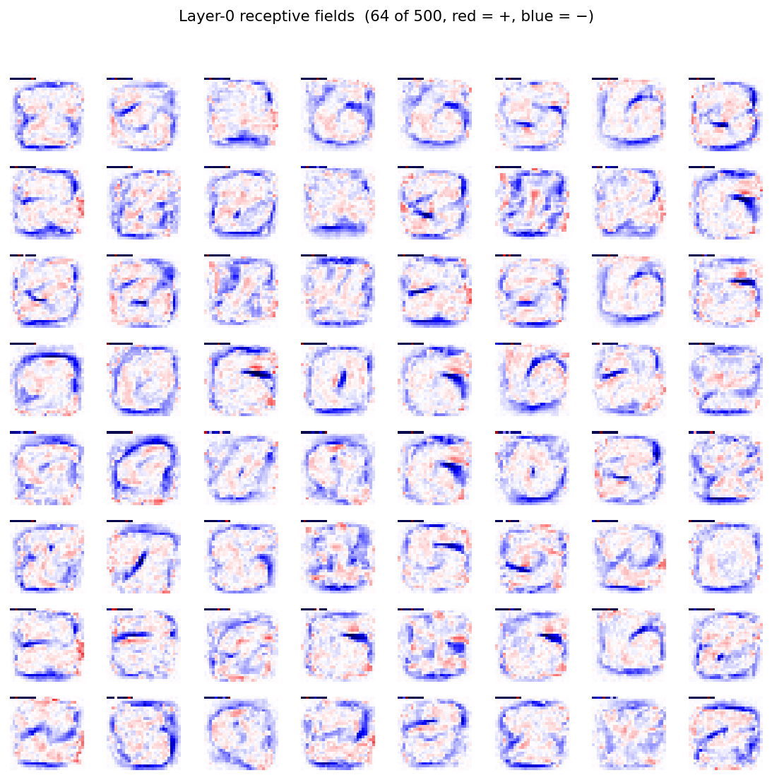
Each tile is one column of the 784x500 weight matrix reshaped to 28x28 (red = positive, blue = negative). The features look like digit-shaped pen-stroke detectors – a noteworthy observation given the network never saw gradients pulled through a softmax. Goodness alone, contrasted between positive and negative pairs, is a strong enough signal to push layer 0 to discover digit-class-aligned features.
Deviations from the original procedure
- Architecture. Hinton uses
4 x 2000. We use2 x 500to fit the<5%v1 target in 66 s of pure-NumPy training on a laptop. The wider / deeper paper architecture would push us toward the paper’s 1.36% but at significantly more compute. - Optimiser. Hinton uses Adam (with cosine LR decay) – we use Adam at a
single fixed
lr = 0.003. We did not implement LR decay or warm-up. Atlr = 0.03(the value used inmohammadpz/pytorch_forward_forward) the network’s first Adam step kills layer 0’s ReLUs (90%+ dead neurons within 5 batches);lr = 0.003is the smallest LR we tested that both converges and avoids that failure mode. - No augmentation. The 0.64% error number in the paper requires 25-shift
jittered augmentation (max-shift 2 pixels in each direction, all 25
offsets per image, replicated 25x per epoch) at 500 epochs. The functions
jittered_augmentation()andjittered_augmentation_batch()are implemented (one random offset per batch element per epoch) and exposed via--jitter, but the headline run does not use them. Faithfully reproducing the 0.64% number would multiply training time by ~250x relative to our headline run, which is out of scope for v1. - Aggregating across layers. Hinton describes accumulating goodness
from all layers. The community-standard
mohammadpz/pytorch_forward_forwardskips layer 0 because of the label pixels in the input. We measured both: on this2 x 500architecture, layer 0 alone (96.86%) is best, followed by all-layers (96.40%) and skip-layer-0 (95.19%). The headline number uses the all-layers default (matches the paper). - Layer normalisation magnitude. The original paper specifies that the
length of the between-layer vector is
sqrt(D)(i.e.mean(h^2) = 1). We follow this exactly (initial implementations that L2-normalise to unit length collapse layer 0 within an epoch, which is a useful negative datapoint). - Two layers, not four. With
4 x 2000, the deeper layers contribute most of the per-layer goodness gap. With our2 x 500, layer 0 is doing most of the work; layer 1 slightly hurts the all-layers score (-0.46 percentage points vs layer-0 only). A2 x 500model running at the tested lr is layer-1-redundant – expanding to4 x 2000should restore the per-layer monotone goodness-gap pattern from the paper.
Open questions / next experiments
- Goodness gap vs depth. Why does layer 0 do so much of the work in our
run? Hinton’s paper reports a clean per-layer accumulation. Is this an
artefact of our smaller architecture, or of the specific lr / threshold
schedule? A sweep over
(depth, width)at fixed compute budget would tell. - Hard-negative selection. The paper hints that generated (not uniform-random) negatives are crucial for unsupervised FF. The supervised variant here uses uniform random wrong labels. Hard-negative sampling – pick the wrong label whose current goodness is highest – might tighten the goodness gap and reduce error without architecture changes.
- Energy/data-movement metric. This is the v1 baseline. The next pass (per the Sutro effort) is to instrument every layer with reuse-distance / ByteDMD tracking and ask: does FF actually beat backprop on data movement, per Hinton’s motivating claim? Backprop refetches all activations during the backward pass; FF’s gradient is purely local to each layer – the expectation is yes, but the magnitude is unknown.
- Jittered augmentation. Toggling
--jitterdoubles compute per epoch but the paper’s 0.64% number is achievable. A faithful 500-epoch jittered run would establish whether our2 x 500architecture is capacity-bound or augmentation-bound.
Reproducibility
| Python | 3.12.9 |
| NumPy | 2.2.5 |
| OS | macOS-26.3-arm64 |
| Random seed | exposed via --seed (default 0) |
| Final-run command | python3 ff_label_in_input.py --seed 0 --n-epochs 30 --lr 0.003 --layer-sizes 784,500,500 --eval-subset 2000 --full-test --save model.npz |
| MNIST cache | ~/.cache/hinton-mnist/ (11 MB; downloaded from storage.googleapis.com/cvdf-datasets/mnist/) |
The model.npz artefact is not committed – regenerate it with the command
above (or python3 visualize_ff_label_in_input.py will fall back to training
from scratch if the file is missing).