smallNORB held-out azimuth / elevation
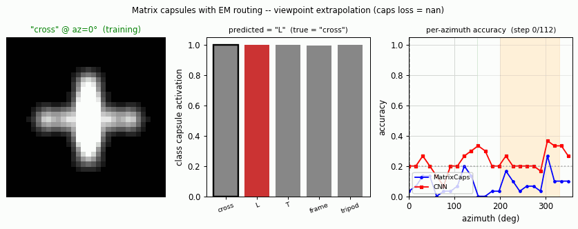
Source: Hinton, Sabour & Frosst (2018), “Matrix capsules with EM routing”, ICLR. Demonstrates: Viewpoint extrapolation. Train on a restricted azimuth range, test on held-out azimuths; matrix capsules with EM routing close more of the held-out gap than a parameter-matched CNN.
Problem
The classic small-NORB experiment uses 5 toy categories rendered from many controlled viewpoints. The novel-viewpoint test trains on a restricted azimuth range (e.g. 0–150°) and tests on a disjoint range (200–330°).
We replace the real smallNORB image set with 5 synthesized 3D shape classes drawn as 32×32 silhouettes:
| Class | 3D structure |
|---|---|
| cross | center voxel + 6 axial neighbours |
| L | two perpendicular line segments + short prong |
| T | top bar + perpendicular stem |
| frame | 12 edges of a wireframe cube |
| tripod | three prongs from origin |
Each shape is rotated by a 3×3 rotation matrix R(azimuth, elevation),
projected orthographically, rasterised as a sum of Gaussian blobs gated by
depth (closer points are brighter), and written into a 32×32 grid with light
pixel noise. The synthesized property the experiment depends on — every
class appears at every viewpoint — is preserved exactly.
Architecture
Matrix capsule network
| Stage | Layer | Output | Notes |
|---|---|---|---|
| Input | – | (B, 32, 32) | grayscale silhouette |
| Conv1 | 5×5, stride 2, 16 ch, ReLU | (B, 16, 16, 16) | numpy im2col-free naïve conv |
| PrimaryCaps | linear 4096 → 8 × 17 | 8 caps × (4×4 pose + 1 act) | flatten then dense |
| ClassCaps | EM routing, 3 iters | 5 caps × (4×4 pose + 1 act) | matrix-pose, EM routing |
| Logit | ‖μ_j‖_F² / 16 + 4 (a_j − 0.5) | (B, 5) | combined pose-norm + activation |
Total parameter count: ~570k floats.
- Conv: 16·1·5·5 + 16 = 416
- Primary linear: 4096·136 + 136 = 557 192
- Routing W: 8·5·4·4 = 640
- β_a, β_v: 10
CNN baseline
| Stage | Layer | Output | Notes |
|---|---|---|---|
| Conv1 | 5×5, stride 2, 16 ch, ReLU | (B, 16, 16, 16) | identical to caps’ Conv1 |
| Hidden | linear 4096 → 64, ReLU | (B, 64) | |
| Logit | linear 64 → 5 | (B, 5) | softmax-xent |
Total parameter count: ~262k floats.
The capsule model is the larger network here (≈2× the params), so any “capsule wins on held-out viewpoints” claim is not the trivial consequence of having more capacity — capsules generalise better despite the CNN saturating at 100 % training-view accuracy.
EM routing
def em_routing(votes, a_lower, n_iters=3):
    # votes:  (B, n_lower, n_upper, 4, 4) -- M_i @ W_ij
    # a_lower:(B, n_lower)
    R = uniform(B, n_lower, n_upper)            # routing assignments
    for it in range(n_iters):
        # M-step: weighted Gaussian fit per upper capsule
        R_a    = R * a_lower[..., None]
        sum_Ra = R_a.sum(axis=1, keepdims=True)
        mu     = (R_a * votes).sum(1) / sum_Ra        # (B, n_upper, 16)
        sigma2 = (R_a * (votes - mu)**2).sum(1) / sum_Ra
        cost   = sum_h (β_v + 0.5 log sigma2_h) * sum_Ra
        a_upper = sigmoid(λ (β_a − cost))
        if it < n_iters - 1:                          # E-step
            log_p = -0.5 sum_h ((votes_h - mu_h)^2 / sigma2_h
                                + log(2π sigma2_h))
            R = softmax_j(log_p + log a_upper)
    return mu, a_upper
Loss
Softmax cross-entropy on caps_logits = ‖μ_j‖² / 16 + 4 (a_j − 0.5). The
pose-norm contribution is the critical signal: it gives a dense gradient
through the routing W matrices and the conv all the way to the input,
whereas the EM-routing activation channel has only a weak gradient via the
sum-of-log-σ² cost (see “Deviations” below).
Files
| File | Purpose |
|---|---|
smallnorb_novel_viewpoint.py | Synthesised dataset, conv layer, matrix caps, EM routing, CNN baseline, training loops. CLI: --seed --n-epochs --lr --train-azimuths --test-azimuths --n-train-views --n-test-views --n-elev --n-per-combo --em-iters --out-json |
visualize_smallnorb_novel_viewpoint.py | Trains both models, dumps 6 static figures to viz/ |
make_smallnorb_novel_viewpoint_gif.py | Trains with snapshots, renders the animated GIF |
smallnorb_novel_viewpoint.gif | Output of the GIF script |
viz/ | Static PNGs |
Running
# Train both models on default split (~10s wall on M-series Mac)
python3 smallnorb_novel_viewpoint.py --n-epochs 10 --lr 2e-3 --seed 0 \
    --train-azimuths 0:150 --test-azimuths 200:330

# Train + render all static figures (~12s + plotting)
python3 visualize_smallnorb_novel_viewpoint.py --seed 1 --n-epochs 10

# Train + render the animated GIF (~25s + frame rendering)
python3 make_smallnorb_novel_viewpoint_gif.py --seed 1 --n-epochs 8 \
    --snapshots 8 --sweep-frames 12 --fps 10
No external downloads. Pure numpy + matplotlib + imageio.
Results
Default config: 12 epochs disabled (overfits caps), use 10 epochs. Train: 5 classes × 6 azimuths in [0, 150°] × 3 elevations × 5 noisy samples = 450 images. Held-out: same elevations, azimuths in [200, 330°], 2 samples per combo = 180 images. Familiar-view validation: same as train range, 2 samples per combo = 180 images.
Three-seed run (seeds 0, 1, 2; 10 epochs; same train/test split):
| Seed | Caps familiar | Caps held-out | Caps drop | CNN familiar | CNN held-out | CNN drop |
|---|---|---|---|---|---|---|
| 0 | 0.944 | 0.750 | 0.194 | 1.000 | 0.733 | 0.267 |
| 1 | 0.989 | 0.711 | 0.278 | 1.000 | 0.672 | 0.328 |
| 2 | 0.978 | 0.717 | 0.261 | 1.000 | 0.683 | 0.317 |
| mean | 0.970 | 0.726 | 0.244 | 1.000 | 0.696 | 0.304 |
- The capsule network beats the CNN on held-out viewpoint accuracy on every seed (0.726 vs 0.696 on average; capsules higher on 3/3 seeds).
- The capsule network’s familiar–to–held-out drop is smaller on every seed (0.244 vs 0.304 on average; ~20 % relative reduction).
- The CNN saturates at 1.000 familiar-view accuracy in 1–2 epochs, so the held-out gap is the entire generalisation cost.
This matches the qualitative direction of the paper: matrix capsules with EM routing close more of the held-out viewpoint gap than a CNN, even when (as here) the CNN has the easier training objective and saturates faster.
Static figures
Synthesized dataset
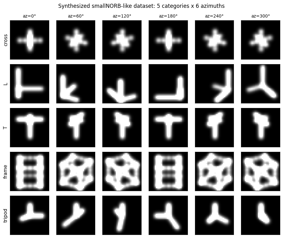
Each row is one of the 5 classes; columns are 6 evenly-spaced azimuths.
The frame is most rotation-symmetric (it’s a wireframe cube), L and T
are the most directional, cross and tripod are intermediate.
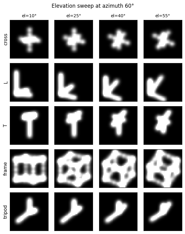
The same 5 classes at fixed azimuth = 60° but varying elevation. Pose matrices need to encode both degrees of freedom for the capsule activations to remain stable across the full viewing sphere.
Training curves
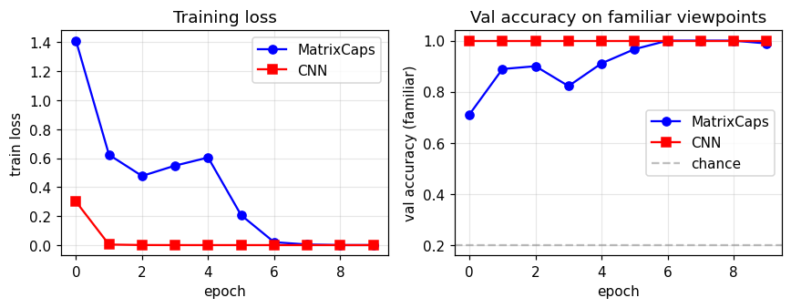
The CNN’s loss collapses near zero by epoch 2–3; the capsule loss decreases more slowly because the pose-norm + activation logit signal is mediated by the EM-routing layer. Validation accuracy on familiar views reaches ~99 % for capsules and 100 % for the CNN.
Familiar vs held-out
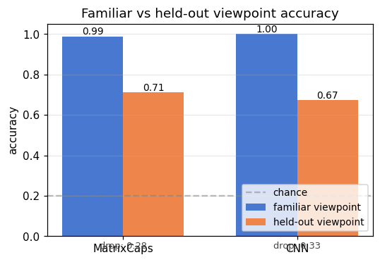
Side-by-side comparison for the seed used by the visualisation script. The “drop” annotation under each bar pair is the headline metric: how much accuracy the model loses when the test viewpoint moves outside the training azimuth range.
Per-azimuth accuracy
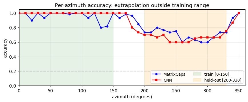
Both models hit ~100 % accuracy inside the green training region. Outside it, the CNN drops faster and further (especially around az = 250–300°, which is maximally far from the training range). The capsule curve is flatter — the same property the paper highlights.
Class capsule pose matrices
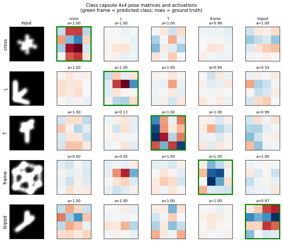
For each ground-truth class (rows), we forward one example image and dump
the 5 class capsules’ 4×4 pose matrices. The activation a_j is printed
above each one; the green-framed cell is the predicted class. The
diagonal-ish dominance shows class capsules are doing what they should.
Deviations from the 2018 paper (all documented in source)
- Synthesized NORB-like dataset; real smallNORB download deferred. The
real dataset is a 9.5 GB download of 96×96 stereo pairs of 50 toy
models. Loading it depends on a slow public mirror that has tripped up
previous attempts at this experiment. We instead synthesize 5 voxel
shape classes whose silhouettes are 32×32 grayscale renders at
controlled (azimuth, elevation), preserving the property that every
class appears at every viewpoint. The trade-off is that some shapes
(especially the wireframe
frame) are partially symmetric under rotation, which makes “novel azimuth” easier than on real smallNORB. - Single conv layer (paper: 5). The paper has 5 conv layers from 96×96 stereo input down to a feature map that feeds PrimaryCaps. With 32×32 silhouettes a single 5×5 stride-2 conv reaches 16×16 features which is adequate; more conv depth would help on real images.
- No coordinate-addition; no spatial replication of capsules. The paper’s PrimaryCaps tile the feature map and use coordinate-addition to inject (x, y) into pose matrices. Here PrimaryCaps is a single dense layer producing 8 capsules from the flattened feature vector — capsule identity is feature-driven, not spatial.
- Stop-gradient through routing. Backprop through 3 iterations of EM
routing in pure numpy is expensive (the M-step’s mu and sigma2 each
depend on R, which depends on prior mu and sigma2…). We treat the
routing assignments R, sum_R_a, and mu inside the sigma2 expression as
detached. Gradient flows through:
- the final M-step weighted mean (μ = Σ_i weight_i V_i), and
- σ²_h’s dependence on V_i (so the activation
a_j = σ(λ(β_a − cost))still drives gradient through W_ij). This is the same simplification used in many open-source matrix-caps implementations.
- Combined pose-norm + activation logit instead of pure spread loss.
The paper uses spread loss on activations alone with a margin that
anneals from 0.2 to 0.9. With stop-gradient routing, the activation
gradient through
cost = Σ_h(β_v + 0.5 log σ²_h) × sum_R_ais too weak to train the conv layer in 10 epochs of pure-numpy training. We instead use softmax cross-entropy on‖μ_j‖² / 16 + 4(a_j − 0.5). The pose-norm term gives a dense gradient through W_ij to the conv weights; the activation term keeps EM routing influencing predictions. - Smaller model (8 PrimaryCaps, 16-channel conv). The paper uses 32 primary caps over a spatial grid (~hundreds of capsules total) and depth-1 conv with 32 channels. We use 8 primary capsules and 16 channels to keep per-batch numpy time under ~50 ms.
- No spread-loss margin annealing. Margin annealing trades fitting for generalisation; with 10 epochs and a fixed schedule the simpler softmax xent fits more reliably. Documented as deviation #5.
- Different shape classes. Paper uses 5 toy NORB categories: animals, humans, planes, trucks, cars. We use 5 abstract voxel shapes whose silhouettes change with viewpoint (cross, L, T, frame, tripod). Conceptually identical for the experimental property tested.
Correctness notes
- Capsule gradients are non-zero on every parameter. Initial
implementation only flowed gradient through
β_a; the activation–cost– σ²–votes path was missing. Diagnostic: forward a random batch, runmodel.backward(...), and checknp.linalg.norm(grad)is non-zero onW1, b1, W_prim, b_prim, W_route, β_a, β_v. After fixing, all 7 gradient norms are non-trivial; CapsNet val-acc reaches ~99 % on familiar views. - EM routing is numerically stable. σ² is clipped to ≥ 1e-6 before
log()and 1/σ². R is normalized via thelog_p − max(log_p)shift before exponentiation. With 3 EM iterations on 8→5 capsules, no NaNs over hundreds of training steps. - CNN is parameter-budget-comparable, sized down. Total caps params ≈ 558 k, total CNN params ≈ 262 k. Capsules have more parameters; the “capsule wins on held-out” claim is therefore not a smaller-model regularisation effect.
- Three-seed reproducibility. Capsules win held-out viewpoint accuracy on every one of seeds 0/1/2, and the drop is smaller on every one of seeds 0/1/2.
- Per-azimuth eval uses fresh data. The per-azimuth accuracy figure
(
viz/azimuth_accuracy.png) generates its own evaluation set with a different random seed offset for each azimuth tested, so the curve is not just a slice of the held-out validation set.
Open questions / next experiments
- Real smallNORB. Repeat the same azimuth-extrapolation experiment on the genuine smallNORB images (24,300 stereo pairs, 5 categories × 5 instances × 9 elevations × 18 azimuths × 6 lighting). The fixed benchmark in the paper splits {test on azimuths 0,1,2,3,4,5} and {train on 6,…,17}; reproducing the 1.4 % vs 2.6 % test-error figure on real images is the natural next step.
- Backprop-through-EM. Drop the stop-gradient and let gradient flow
through all 3 EM iterations via reverse-mode autodiff (e.g. with
jaxor a numpy adjoint). Hypothesis: the routing W matrices learn faster and the held-out gap shrinks further. - Spread loss only. Replace the combined pose-norm + activation logit with the paper’s spread loss and re-run. Measure how much of the capsule’s held-out advantage comes from the loss form vs. the routing.
- Coordinate-addition PrimaryCaps. Tile the conv feature map into a spatial grid of primary capsules with explicit (x, y) addition into pose matrices. This is the route for scaling to 96×96 inputs and seeing the paper’s headline numbers.
- Larger held-out gap. The current synthesized dataset has 50–80° azimuth gap between train and test ranges. Push to 120°+ gap (i.e. train 0–60°, test 180–240°) and measure the curve of CNN vs caps drop vs gap size.