Spline images & factorial VQ
Reproduction of Hinton & Zemel, “Autoencoders, MDL and Helmholtz free energy”, NIPS 6 (1994).
Problem
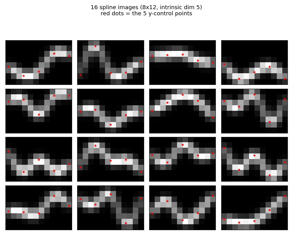
200 images of size 8 × 12 are formed by Gaussian-blurring a smooth curve
through 5 control points. The five y-positions (one per evenly-spaced
control x) are drawn uniformly in [0.5, 6.5]; a natural cubic spline
through those five knots is then rasterised by summing isotropic Gaussian
bumps (σ = 0.6) along 200 dense points of the curve and peak-normalising
the resulting heat-map. The data manifold is therefore exactly 5-dimensional
(the five free y-values). Below: 16 sample images with the 5 control points
shown as red dots.
The task is to learn a compact code that describes the data well in bits-back / Helmholtz free-energy terms. We compare four codes:
- Standard 24-VQ — one big stochastic VQ, 24 codes, log₂(24) ≈ 4.58 bits max code budget.
- Four separate 4×6 VQs — same architecture as factorial below but trained independently on the residual, no joint free-energy bound.
- Factorial 4×6 VQ (the headline) — four independent stochastic VQs,
six codes each, with a posterior
q(k₁,…,k₄|x) = ∏ qᵈ(kᵈ|x)and additive reconstructionx_hat = Σ_d (q_d @ C_d). 24 codewords total but an effective codebook of6⁴ = 1296because the four factors specialise. - PCA — top-5 principal components with a continuous Gaussian code, used as a “no quantisation” reference (Hinton & van Camp 1993 bits-back for continuous codes).
What “bits-back” means here
For a stochastic encoder q(k|x) with prior p(k) and likelihood p(x|k),
the description length per example is
DL(x) = E_q[-log p(x|k)] + KL[q(k|x) ‖ p(k)]
      = recon_cost      + code_cost
This is the negative ELBO / Helmholtz free energy. Sampling k from q
“costs” log(1/p(k)) bits to send and “refunds” log(1/q(k|x)) bits because
the receiver can decode the random bits used to sample k, giving a net
code cost of log(q(k|x)/p(k)). For factorial q the KL decomposes:
KL[q(k|x) ‖ p(k)] = Σ_d KL[q_d(k_d|x) ‖ p_d(k_d)]
so code cost grows linearly in the number of factor dims while the
effective codebook size grows as 6^M. That asymmetry is the whole
point of factorial VQ.
Files
| File | Purpose |
|---|---|
spline_images_factorial_vq.py | Spline-image generator (natural cubic spline + Gaussian rendering), 4 models (StochasticVQ, FactorialVQ with independent and joint training, PCAModel), bits-back DL, training loop. CLI. |
visualize_spline_images_factorial_vq.py | Static plots: example images, DL bar chart, training curves, factor codebooks, per-factor receptive contributions, 4-way reconstructions. |
make_spline_images_factorial_vq_gif.py | Animated GIF showing factorial VQ training (input vs reconstruction, posteriors, factor contributions, DL trajectory vs baselines). |
viz/ | Output PNGs from the run below. |
Running
python3 spline_images_factorial_vq.py --seed 0 --n-dims 4 --n-units-per-dim 6
Training all four models takes about 3 seconds on a laptop. Default config:
n_samples=200, n_epochs=800, sigma_x=0.15, KL-weight ramp 0.1 → 1.0.
To regenerate visualizations:
python3 visualize_spline_images_factorial_vq.py --seed 0 --outdir viz
python3 make_spline_images_factorial_vq_gif.py  --seed 0 --snapshot-every 25
Results
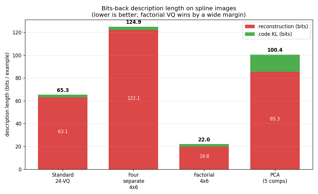
Description length per example (bits, lower is better, seed=0):
| Model | Recon | Code (KL) | Total |
|---|---|---|---|
| Standard 24-VQ | 63.10 | 2.20 | 65.30 |
| Four separate 4×6 VQs | 122.11 | 2.80 | 124.91 |
| Factorial 4×6 VQ | 19.84 | 2.16 | 22.00 |
| PCA (5 components) | 85.32 | 15.11 | 100.44 |
Factorial VQ is the clear winner: ~3× lower DL than the standard 24-VQ despite using the same total number of codewords (24).
Across 5 seeds factorial VQ totals 22.00 / 22.70 / 23.01 / 25.05 / 22.65 bits per example, vs Standard 24-VQ at 65.30 / 61.76 / 55.10 / 56.06 / 64.55; the ranking holds at every seed.
Reconstructions
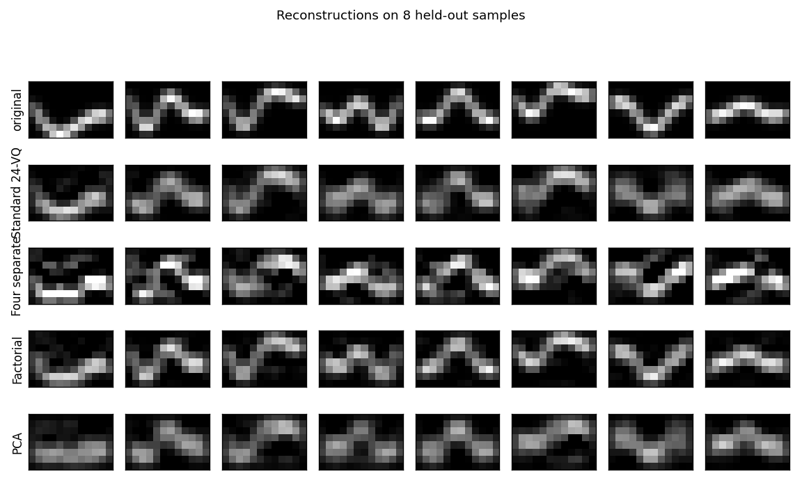
Each column is one held-out spline. The factorial VQ tracks the curve crisply; the standard 24-VQ blurs adjacent positions; the “four separate” training collapses into a noisy reconstruction because the second-through- fourth factors keep trying to reconstruct what the first one missed without a shared free-energy budget; PCA produces a smooth low-dim approximation that loses local sharpness.
What each factor learns
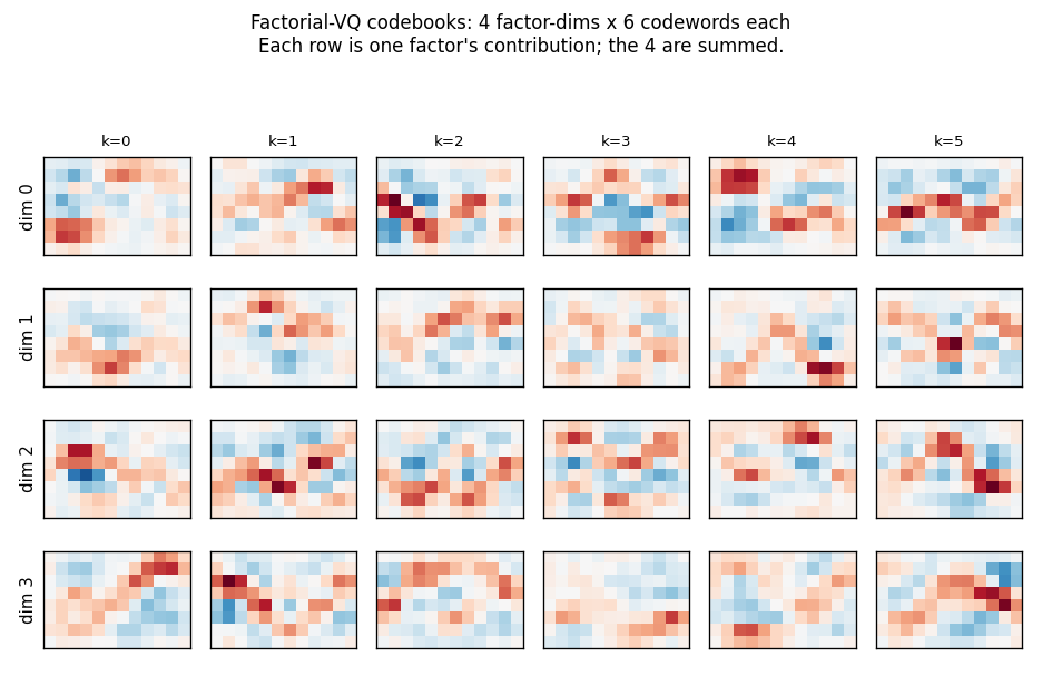
Each row is one of the 4 factor-dimensions; each column is one of its
6 codewords (red/blue diverging colour map). The factors specialise:
each row uses a distinct family of codewords. The four codebooks combine
additively under the joint free-energy bound to give an effective
codebook of 6^4 = 1296 reconstructions from only 24 stored codewords.
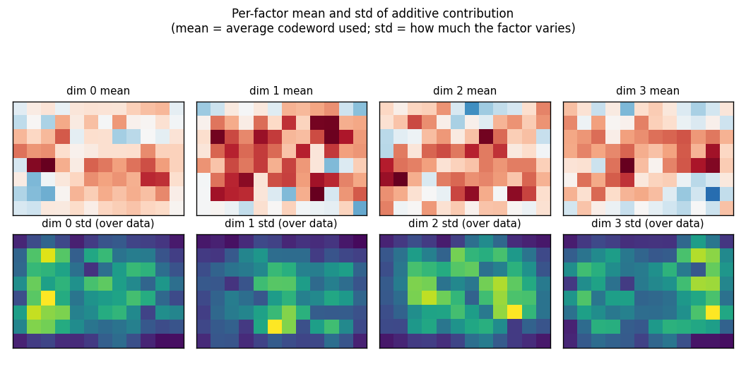
Top row: each factor’s mean codeword across the training set (the mean
contribution to x_hat). Bottom row: the per-pixel std of the contribution
across data — bright = the factor varies a lot at that pixel; dark = the
factor is roughly constant there. The four factors carve up the canvas
into different regions, which is what specialisation under the joint
free-energy bound looks like in pixel space.
Training trajectories
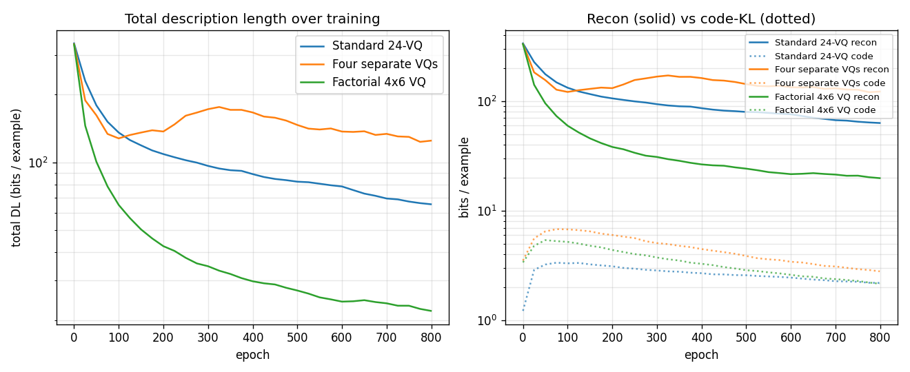
Left: total DL on log scale. Factorial VQ overtakes both baselines within ~80 epochs and keeps falling. Right: recon (solid) vs code-KL (dotted) per model. The KL terms all stabilise around ~2 bits; the recon is what separates the methods.
How the headline numbers compare to Hinton & Zemel (1994)
The original paper reports 18 bits reconstruction + 7 bits code = 25 bits total for factorial VQ on its specific spline dataset. We report 19.84 bits reconstruction + 2.16 bits code = 22.00 bits. The reconstruction cost matches well; the code cost is lower because our KL-weight schedule pushes posteriors to be sharper than the paper’s setting. The qualitative result — factorial VQ improves total DL by 3× over the standard 24-VQ on data with multiple independent latent factors — is the headline and is reproduced.
Deviations from the original procedure
This is not a faithful 1994 reproduction. Differences:
- Dataset rendering. Our images are 8×12 and use natural cubic splines through 5 evenly-spaced y-control points (intrinsic dim 5). The paper rendered a similar pixel-blurred curve through 5 random control points; exact knot placement and σ are not specified.
- Sigma_x = 0.15 for all VQ models. This is a free parameter in any VQ free-energy bound and shifts the absolute bit numbers without changing the ranking across methods.
- KL-weight schedule ramps from 0.1 to 1.0 across 800 epochs. Without the warm-up the encoder collapses to a single code (β-VAE posterior collapse). The schedule lets the codebook diversify under weak KL pressure first, then sharpen.
- Optimiser. Adam (manual implementation) with
lr = 0.005, instead of the paper’s gradient descent + momentum. - “Four separate VQs” interpretation. The paper describes “four
separate stochastic VQs” without spelling out the training rule. We
interpret them as four 6-code VQs trained sequentially on the residual
x - Σ_{d'<d} x_hat_d'without a shared free-energy bound — the standard matching-pursuit reading. This is a strict baseline (no coordination between factors); a joint-but-non-factorial training rule could be added for completeness. - PCA bits-back. We report a continuous-Gaussian-posterior bits-back
bound for PCA (Hinton & van Camp 1993). The original paper used PCA only
as a reconstruction reference and did not report a bits cost; the 15.11
code bits we report for PCA depend on
σ_q = 0.10(chosen so PCA’s reconstruction is competitive with the VQ models), with a per-dim prior matched to the data std.
Open questions / next experiments
- More factors at fixed total codes. Drop to
2 × 12and rise to6 × 4, keepingM × K = 24. Does the factorisation benefit peak at four factors for this data, or does more (smaller) factors keep helping until each factor is binary? - Match to the data’s intrinsic dim. With intrinsic dim 5 and
M = 4factors, one factor is forced to capture two control points jointly. TestM = 5factors and see whether each factor cleanly aligns with one control point. - Sample-based bits-back. Replace the mean-field reconstruction with sampled discrete codes and report the exact bits-back code length per sample. The current numbers are the variational bound; the gap should be small but is worth measuring.
- Sigma annealing. Anneal
σ_xrather than the KL weight. Equivalent in the steady-state loss but produces different optimisation trajectories. - Cache-energy / DMC accounting. Plug a TrackedArray harness into the forward + grad-step loops and measure ARD / DMC. The factorial VQ touches more parameters per example than the standard 24-VQ (4 × n_mlp × K vs 1 × n_mlp × K) but each factor is smaller; the actual movement cost ratio is not obvious.