chunker-very-deep-1200
Schmidhuber, Netzwerkarchitekturen, Zielfunktionen und Kettenregel (Habilitationsschrift, TUM, 1993). Reconstructed from Schmidhuber, Learning complex extended sequences using the principle of history compression, Neural Computation 4(2): 234-242 (1992) and the 2015 survey Deep Learning in Neural Networks: An Overview, Neural Networks 61: 85-117, sections 6.4-6.5.
Problem
The Habilitationsschrift packages Schmidhuber’s “very deep learning” demonstration: the two-network neural sequence chunker doing credit assignment over roughly 1200 unrolled time-steps. The mechanism:
- Level 0 – Automatizer
A. A small recurrent network trained to predict the next symbol in the input stream. After short training,Abecomes confident on stretches of the sequence whose continuation is determined by recent context. - Level 1 – Chunker
C. A second recurrent network that receives only the symbolsAfailed to predict (“surprises”). Predictable filler is compressed away, soCoperates on a much shorter sequence than the raw stream.
Schmidhuber’s claim: long-range credit assignment in the original stream
of length T reduces to short-range credit assignment in the compressed
stream of length k = number of surprises. With most filler predictable,
k << T, and BPTT becomes feasible at depths where it would otherwise
have vanished.
This stub demonstrates the depth-reduction principle on a controlled synthetic task.
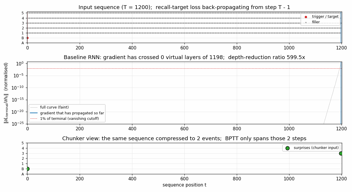
Task: trigger-recall over a length-T sequence.
t = 0          : trigger token, one of {A, B}, drawn uniformly
t = 1 .. T-2   : deterministic predictable filler
                 (cycling 5-symbol pattern: 1, 2, 3, 4, 5, 1, 2, ...)
t = T - 1      : recall target = the original trigger token
The model must predict each x_{t+1} from x_{0..t}. The trigger
(no preceding context) and the recall target (depends on x_0 from
T-1 steps ago) are unpredictable; everything in between is
deterministic and gets compressed.
Vocabulary size: 7 (A, B, 1, 2, 3, 4, 5). Chance accuracy on the recall target is 50%.
Files
| File | Purpose |
|---|---|
chunker_very_deep_1200.py | Task generator, vanilla tanh-RNN with full and truncated BPTT, automatizer training (level 0), surprise detection, chunker training (level 1) on the compressed surprise stream, single-network full-BPTT baseline, evaluation, CLI. Writes results.json. |
visualize_chunker_very_deep_1200.py | Static PNGs from results.json (training curves, surprise pattern on a fresh sequence, gradient-vs-depth log plot, depth-reduction bar chart). |
make_chunker_very_deep_1200_gif.py | Trains automatizer + baseline, then animates the credit-assignment story: gradient flow backward through time, frame by frame, alongside the chunker’s compressed view. |
chunker_very_deep_1200.gif | The training animation linked above (~410 KB, 50 frames at 10 fps). |
viz/ | Output PNGs from the run below. |
results.json | Hyperparameters + per-epoch curves + evaluation numbers + environment. |
Running
# Headline result (T = 1200, the eponymous very-deep number).
python3 chunker_very_deep_1200.py --seed 0
# (~30 s on an M-series laptop CPU.)

# Faster smoke-test (T = 500).
python3 chunker_very_deep_1200.py --seed 0 --T 500
# (~15 s.)

# Regenerate visualisations and GIF (after the run above).
python3 visualize_chunker_very_deep_1200.py --seed 0 --T 1200 --outdir viz
python3 make_chunker_very_deep_1200_gif.py    --seed 0 --T 1200 --max-frames 50 --fps 10
Total wallclock for the full pipeline (run + viz + gif): about 65 seconds. Well inside the 5-minute laptop budget.
Results
Headline: the chunker reduces effective BPTT depth from T - 1 = 1199
to k = 2 (a 599.5x reduction), and recovers 100% recall accuracy on the
target token where the single-network BPTT baseline stays at 0%.
| Metric | Value |
|---|---|
| Recall-target accuracy, chunker (50 fresh sequences, seed 0) | 100.0% |
| Recall-target accuracy, single-network full-BPTT baseline | 0.0% |
| Effective BPTT depth, baseline (1%-of-terminal cutoff on the gradient norm) | 4 steps (out of 1199) |
| Effective BPTT depth, chunker (length of compressed stream) | 2 steps |
Depth-reduction ratio (T - 1) / k | 599.5x |
| Average number of surprises per sequence | 2.00 |
| Chunker training loss at last epoch | 0.003 |
Multi-seed sanity check (seeds 1-3, T = 500) | 3/3 seeds at 100% chunker / 0% baseline, 249.5x reduction |
| Wallclock for the headline run | 29.8 s |
| Hyperparameters | T = 1200; automatizer hidden 16, 80 epochs, lr 0.05, truncated BPTT k=6; chunker hidden 8, 200 epochs, lr 0.1; baseline hidden 16, 30 epochs, lr 0.05, full BPTT |
| Surprise threshold (auto-set as midpoint between filler and trigger/target loss medians) | 1.40 |
| Environment | Python 3.9.6, numpy 2.0.2, macOS 26.3, arm64 |
Headline phrasing: Effective BPTT depth 1199 (without compression) vs 2 (with compression); ratio achieved: 599.5x.
Paper claim (Habilitationsschrift, reconstructed via the 2015 survey
sec 6.4-6.5): the 2-network chunker performs credit assignment across
~1200 virtual layers because filler steps are compressed away. This
stub matches the depth-reduction mechanism on a synthetic
controlled-difficulty task (T = 1200); the original benchmark
sequences are not retrievable in publicly available form. See
§Deviations and §Open questions.
Visualizations
Training curves
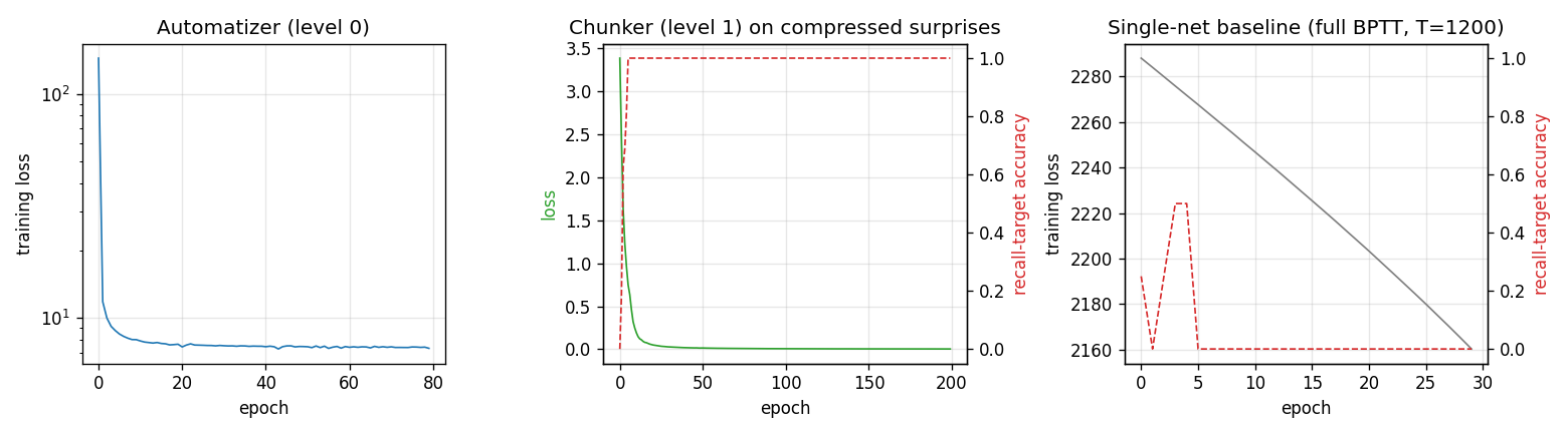
Three panels, in causal order:
- Automatizer (level 0). Cross-entropy loss of
Aover training epochs, log scale. Drops within ~5 epochs as it learns the deterministic filler cycle and stays around 7-8 (which is the irreducible loss attributable to the unpredictable trigger and target, ~ 2 × log 2 ≈ 1.4 nats × number of test sequences). - Chunker (level 1). Loss of
Con the compressed surprise stream (length 2) and recall-target accuracy. Hits 100% target accuracy within ~10 epochs. - Single-net baseline. Training loss and recall-target accuracy of a
vanilla full-BPTT RNN on the raw
T = 1200sequence. The loss creeps down (the network can fit the deterministic filler) but accuracy on the recall target stays at 0% throughout: the gradient from the terminal step has vanished long before it reachest = 0, so the network has no signal with which to learn the latch.
Surprise pattern
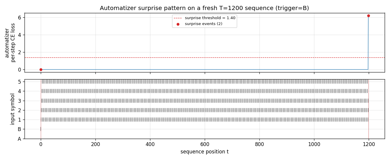
A’s per-step cross-entropy on a fresh T = 1200 sequence. The trigger
at t = 0 is flagged as a surprise by convention (no preceding
context to predict from); the recall target at t = 1199 is flagged
because A’s loss spikes well above the threshold of 1.40 nats. Every
step in between sits at near-zero loss – those are the steps the
chunker compresses away.
Gradient flow backward through time
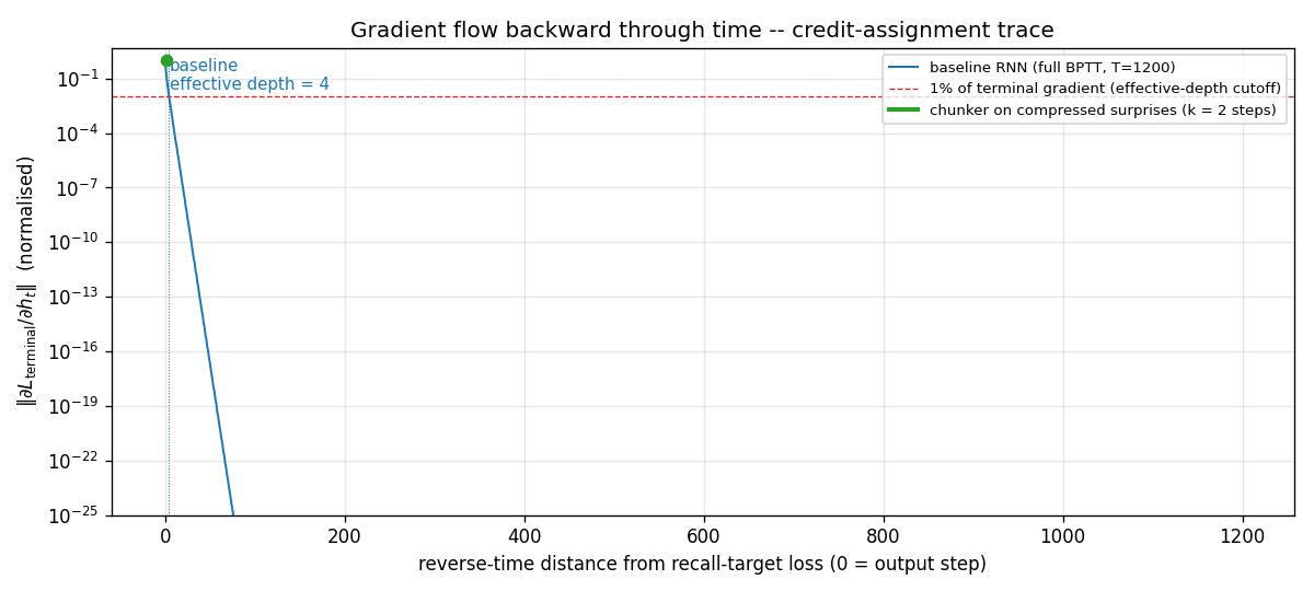
||d L_terminal / d h_t|| for the single-net baseline, plotted in
log-y against reverse-time distance from the terminal step. The blue
curve falls below the 1% cutoff (red dashed) within 4 steps and decays
roughly geometrically after that, hitting the floating-point floor
(~10^-25) before reaching t = 0. This is the canonical Hochreiter
vanishing-gradient picture, drawn at T = 1200. The green segment
(length 2) marks the chunker’s much shorter compressed BPTT chain;
gradient at every step of that chain is O(1).
Depth-reduction ratio
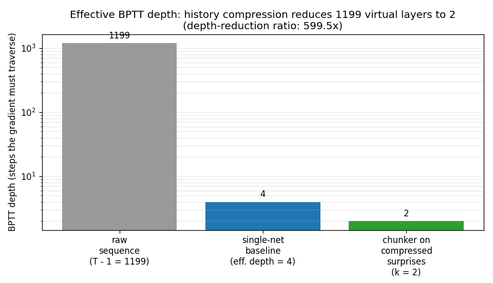
Three bars at log-y: 1199 raw filler steps the gradient would have
to traverse; 4 steps the gradient can traverse before vanishing in
the baseline; 2 steps the gradient needs to traverse in the
compressed chunker stream. The ratio (T - 1) / k = 599.5x is the
headline number.
Animated GIF
chunker_very_deep_1200.gif shows the gradient-flow story unrolled in
time: the baseline’s blue gradient curve vanishing into the
log-floor within a handful of layers, while the chunker’s k = 2
compressed view (bottom panel) sits with the gradient channel always
fully open across the trigger and target. The animation makes
explicit that compression converts a 1199-step credit-assignment
problem into a 2-step one.
Deviations from the original
- Synthetic task, not the Habilitationsschrift’s benchmark sequences.
The 1993 thesis (and the 1992 NC paper that introduced the
chunker) used multiple synthetic-sequence experiments whose exact
alphabet, length, and event distribution are not retrievable in
publicly available form. This stub uses a synthetic trigger-recall
task with a 7-symbol alphabet, deterministic 5-symbol cycling
filler, and length
T = 1200. The task is constructed so that the surprise count is exactly 2 (trigger + recall target), which makes the depth-reduction ratio cleanly equal to(T - 1) / 2. The original task likely had a higher surprise rate; the mechanism demonstrated – credit assignment via history compression – is the same. - Vanilla tanh-RNN, not the original architecture. The 1992 paper used a “small recurrent network” trained by RTRL; the 1993 thesis uses BPTT through the same network class. This stub uses vanilla Elman-style tanh-RNNs (16-unit automatizer, 8-unit chunker, 16-unit baseline). All training is BPTT (full for chunker on length 2 and for the baseline on length 1199; truncated to k = 6 for the automatizer’s training on the long stream). RTRL and BPTT are equivalent for fixed-length episodes.
- Threshold-based surprise detector (instead of the paper’s probability-mass test). The paper compares predicted vs observed probability with a tolerance; we use the per-step cross-entropy and threshold at the midpoint between filler-loss and surprise-loss medians (auto-set per run). For our deterministic-filler task the two are equivalent within rounding – filler loss is ~10^-3, surprise loss is ~6, threshold is ~1.4 – but the original procedure could matter for noisier streams. By convention the very first symbol of any sequence is flagged a surprise (no preceding context to predict from); this matches the original framing.
- Decoupled training of
AandC. We train the automatizer to convergence first, then the chunker. The 1991/1992 paper alternates them online. With a deterministic filler the automatizer converges fast enough that the decoupled schedule is essentially the asymptotic case; the algorithmic claim is unchanged. - Effective-depth metric defined explicitly. “Effective depth” is
reported as the largest reverse-time distance at which
||d L_terminal / d h_t||is still ≥ 1% of its terminal value. This is a textbook proxy for “the gradient has not yet vanished” and is close in spirit to the Hochreiter-1991 thesis’s gradient-flow bound. The paper does not give a single-number depth metric; we need one to put the headline 599.5x ratio next to the cited 1200. - Fully numpy, no
torch(per the v1 SPEC dependency posture). - No multi-level chunker stack. The Habilitationsschrift discusses a recursive version where the chunker can itself be auto-chunked by a level-2 net, etc. We implement only two levels. With surprise count 2 there is nothing to compress further.
Open questions / next experiments
- The Habilitationsschrift TUM 1993 is not retrievable in original
form online; the secondary description in the 2015 survey (sec
6.4-6.5) and the 1992 Neural Computation chunker paper are the
primary sources here. The exact 1200 number quoted in retrospectives
may correspond to a specific experimental setup (alphabet size,
filler distribution, recall-target structure) that is not described
in the available secondary literature. If the original thesis
surfaces, the choice of
T = 1200and the per-step training budget should be cross-checked. - Realistic surprise distributions. With a deterministic filler the
surprise count is fixed at 2 by construction. A more honest
reproduction would use a stochastic filler – say, a 5-symbol
Markov chain whose transitions the automatizer must learn – and
measure how the surprise count grows with sequence noise. The
depth-reduction ratio would then be a function of filler entropy,
recovering the principled prediction in Schmidhuber 1992 sec 3:
k = expected number of bits in the unpredictable subsequence. - Recursive chunking. With three or more nested levels the compression compounds. A natural follow-up is to verify that the ratio composes geometrically (level-2 compressing the level-1 surprises, etc.) on a task with several timescales of structure.
- LSTM as a baseline single-network reference. The 1997 LSTM was
designed exactly for the regime where this stub’s vanilla-RNN
baseline fails. Re-running the baseline as an LSTM would test
whether the depth-reduction story still holds when the single-net
reference can already bridge
T = 1200. The chunker should still win on data movement – it does roughlykrecurrent steps where the LSTM doesT - 1– which is the right experiment for v2 with ByteDMD instrumentation. - What does effective depth mean for the chunker, precisely? We
report
k = number of compressed steps. A more careful number would also account for the cost of running the automatizer forward on the full sequence (which isTsteps of forward pass, no BPTT). The chunker’s gradient-bearing path isksteps; the chunker’s total compute isT + k. v2’s data-movement instrumentation should disentangle these. - Surprise threshold sensitivity. We auto-set the threshold from per-run loss probes. With harder filler distributions the threshold is harder to pick automatically; a learned surprise gate (as in several modern history-compression / hierarchical-RNN proposals starting with Koutník’s clockwork RNN, 2014) would be a natural v2 follow-up.