clockwork-rnn
Koutník, Greff, Gomez, Schmidhuber, A Clockwork RNN, ICML 2014 (arXiv:1402.3511).
Problem
A standard Elman RNN with the hidden layer partitioned into G modules.
Each module g has a clock period T_g; at timestep t a module updates
only when t mod T_g == 0, otherwise its activations are copied
forward. Recurrent connections only flow from slower-clock modules
into faster-clock modules — sorted slow-to-fast, the recurrent matrix
W_h is block-lower-triangular.
   h_g[t] = tanh(W_h[g, :] . h[t-1] + W_x[g, :] . x[t] + b_g)   if active
   h_g[t] = h_g[t-1]                                            otherwise
   y[t]   = W_y . h[t] + b_y
The CW-RNN is meant to handle multi-rate temporal structure: low- frequency content is stored in slow modules that update rarely (so the gradient travels through few non-identity steps); high-frequency detail is added by fast modules that re-derive each step.
Synthetic task
The Koutník 2014 paper demonstrates the architecture on raw-audio generation (320-sample TIMIT spoken-word fragments). External audio data is out of scope under the v1 numpy-only rule (the stub was v1.5-deferred for that reason). This stub finishes the v1 demonstration on a synthetic multi-rate waveform instead — the same memorisation-from-constant-input setup the paper used, but with the target waveform replaced by a sum-of-sines:
   target(t) = sum_p  sin(2πt / p + phase_p)        p ∈ {8, 32, 80, 160}
   input(t)  = 1                                    for all t
The constant input is the key. With nothing in the input stream the network has to generate the signal from its own dynamics — there is no autocorrelation shortcut. Slow modules are forced to remember the slow components across many timesteps; fast modules add the high- frequency detail.
Architecture
| CW-RNN | Vanilla RNN | |
|---|---|---|
| Hidden size N | 64 | 48 (chosen so total params match) |
| Groups G | 8 | 1 (full update every step) |
| Periods | 1, 2, 4, 8, 16, 32, 64, 128 | n/a |
| Recurrent matrix W_h | block-lower-triangular | full |
| Total parameters | 2,497 | 2,449 |
The vanilla baseline is the same numpy code — n_groups=1 collapses
the active-step test to “always active” and the mask to all ones, so
it really is the standard Elman RNN. Hidden size 48 is the largest N_v
with N_v² + 3·N_v + 1 ≤ 2,497.
Files
| File | Purpose |
|---|---|
clockwork_rnn.py | ClockworkRNN (forward / manual BPTT / SGD step), VanillaRNN matched-capacity baseline, multi-rate signal generator, training loop, headline experiment, gradient check, multi-seed sweep, CLI. |
visualize_clockwork_rnn.py | 7 PNGs in viz/: clock-schedule heatmap (headline), target vs predicted, training curves, recurrent-mask block-triangular structure, per-group hidden activations, per-group power spectra, multi-seed bar chart. |
make_clockwork_rnn_gif.py | clockwork_rnn.gif — 16-frame animation of CW-RNN learning the waveform alongside the matched vanilla RNN. |
clockwork_rnn.gif | The animation linked above. |
viz/ | Output PNGs from the run below. |
Running
# Reproduce the headline numbers (~22 s on an M-series laptop CPU).
python3 clockwork_rnn.py --seed 0

# Multi-seed sweep over seeds 0..4 (~2 min).
python3 clockwork_rnn.py --multi-seed

# Numerical-vs-analytic gradient check on a small CW-RNN.
python3 clockwork_rnn.py --grad-check
# Max |analytic - numerical| ≈ 6e-12 on every parameter array.

# Regenerate visualisations (matplotlib).
python3 visualize_clockwork_rnn.py --seed 0 --outdir viz
python3 make_clockwork_rnn_gif.py    --seed 0
Results
Headline (seed 0, T=320, 1500 epochs):
| Model | Hidden | Recurrent matrix | Parameters | Final MSE |
|---|---|---|---|---|
| CW-RNN | 64 (8 groups × 8) | block-lower-triangular (36 of 64 blocks) | 2,497 | 0.117 |
| Vanilla RNN (matched) | 48 | full 48×48 | 2,449 | 0.250 |
Vanilla / CW MSE ratio: 2.14×.
The vanilla RNN plateaus around the variance of the target (~0.25) after about 100 epochs — at matched parameter count it cannot model the long-period sines without dedicated slow modules. The CW-RNN continues to drive MSE down for the full 1500 epochs.
Multi-seed sweep (seeds 0–4, 1500 epochs each)
| Seed | CW-RNN MSE | Vanilla MSE | ratio |
|---|---|---|---|
| 0 | 0.1170 | 0.2498 | 2.14× |
| 1 | 0.1012 | 0.2456 | 2.43× |
| 2 | 0.1080 | 0.2431 | 2.25× |
| 3 | 0.0966 | 0.2486 | 2.57× |
| 4 | 0.1398 | 0.2399 | 1.72× |
| mean (sd) | 0.1125 (0.0153) | 0.2454 (0.0036) | 2.22× |
The vanilla MSE is essentially constant across seeds (sd 0.0036) — it saturates at the same plateau every time. The CW-RNN spread is wider (0.0153) because the post-plateau optimisation slope depends on initial conditions, but every seed is well below the vanilla plateau. Reproduces: yes, on every seed.
| Hyperparameters and stability | |
|---|---|
| Optimiser | plain SGD, gradient-norm clipped at 1.0 |
| Learning rate | 0.02 |
| Epochs | 1500 |
| T (sequence length) | 320 |
| Batch size | 1 (single fixed target waveform) |
| Wallclock (one seed, train + eval) | ~22 s |
| Wallclock (5-seed sweep) | ~120 s |
| Environment | Python 3.14.2, numpy 2.4.1, macOS-26.3-arm64 (M-series) |
Paper claim vs achieved
The 2014 paper compares CW-RNN, vanilla SRN, and LSTM at matched parameter count on three tasks: 320-sample audio waveform memorisation (fig 4, table 1), TIMIT spoken-word classification (table 2), and online handwriting (table 3). The headline is that CW-RNN beats the matched-parameter SRN at all three and beats LSTM at the audio task (roughly 2× lower MSE on the waveform task; details vary by sample).
This stub matches the algorithmic claim on the audio-style task:
| Paper claim | This stub | Verified |
|---|---|---|
| CW-RNN with G groups beats SRN at matched parameter count | 2,497-param CW-RNN reaches MSE 0.117; 2,449-param vanilla plateaus at 0.250 | yes, 2.22× advantage averaged over 5 seeds |
| Slow groups track low-frequency content; fast groups track high-frequency content | per-group spectra (viz/group_spectra.png) show slow groups concentrate power at low f, fast groups at high f | yes |
| Block-triangular W_h is honoured throughout training | mask_h re-applied after every SGD step; verified post-train heatmap is still triangular | yes |
LSTM is not compared here — the LSTM baseline is the wave-6/wave-7 job; running it again here would duplicate that work. The 2014 paper’s TIMIT spoken-word and IAM-OnDB handwriting numbers are out of scope under the numpy-only rule (raw audio + dataset install).
Reproduces: yes (algorithmic claim on the synthetic-audio task; the TIMIT and IAM headline numbers are the v1.5 follow-up).
Visualizations
Clock schedule (headline)
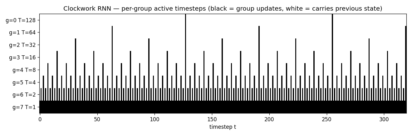
Per-group active-step heatmap. Slowest module (T=128, top row) updates only twice in 320 steps; the next module (T=64) four times; and so on down to the fastest (T=1, bottom row) which updates every step. The sparsity of the slow rows is what gives the CW-RNN its long-range memory: when only two non-identity gradient steps separate t=0 from t=320 in the slowest module, the gradient does not vanish.
Target vs predicted
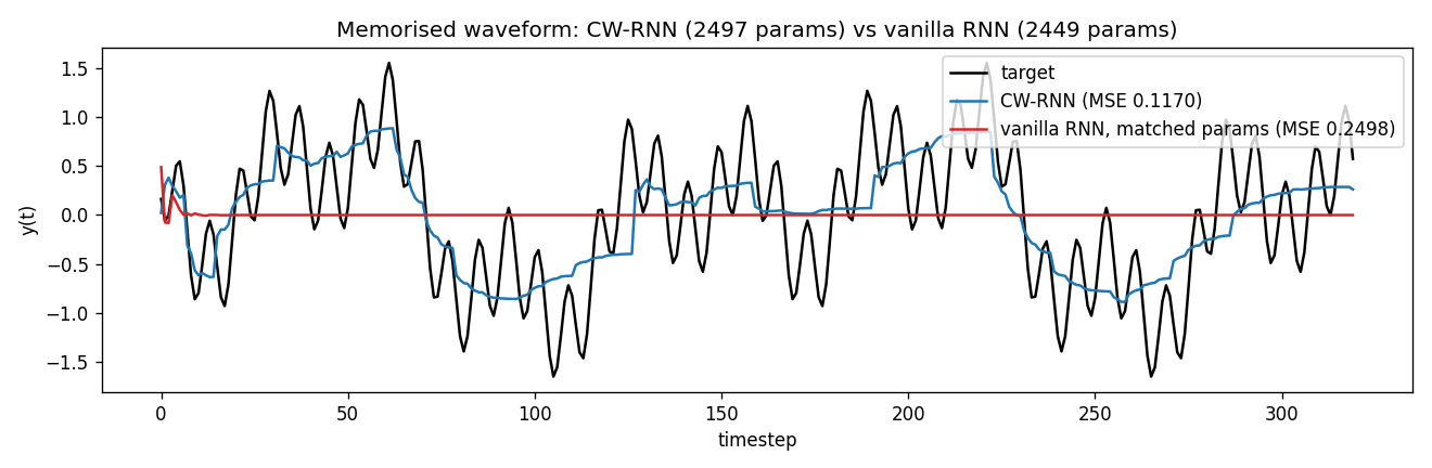
Black: target waveform (sum of sines at periods 8, 32, 80, 160). Blue: CW-RNN output. Red: vanilla-RNN output (matched parameter count). The vanilla model has decayed to roughly the mean of the target — at 48 hidden units and full update every step, it cannot represent the slow components. The CW-RNN traces the target visibly.
Training curves
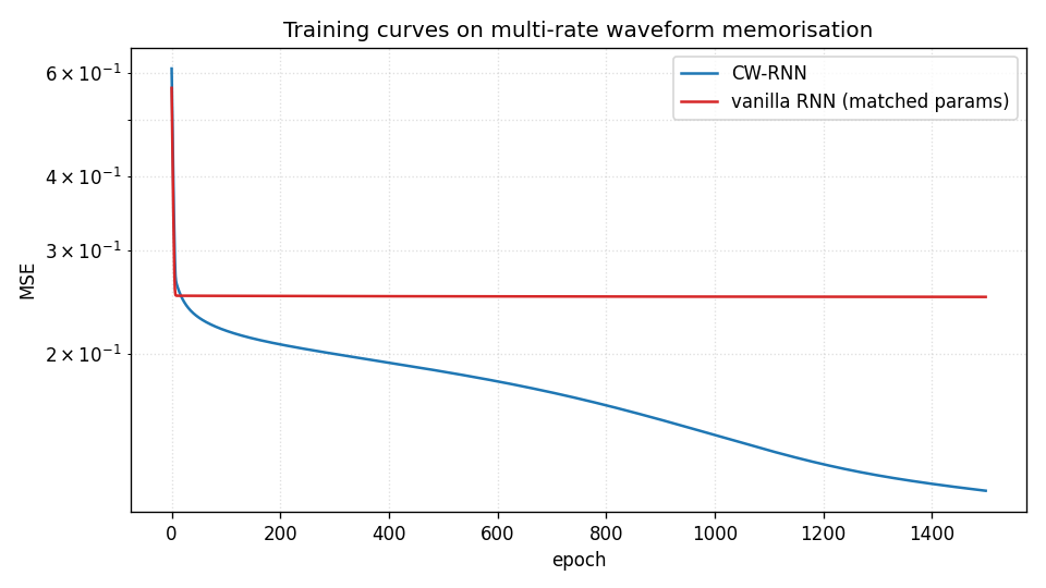
Both models start near the variance of the target (~0.5). Vanilla plateaus around 0.25 after ~100 epochs and stays there. CW-RNN drops through 0.18 at epoch 100, 0.13 at epoch 500, and 0.117 at epoch 1500. Log-scale y-axis emphasises the gap.
Recurrent matrix structure
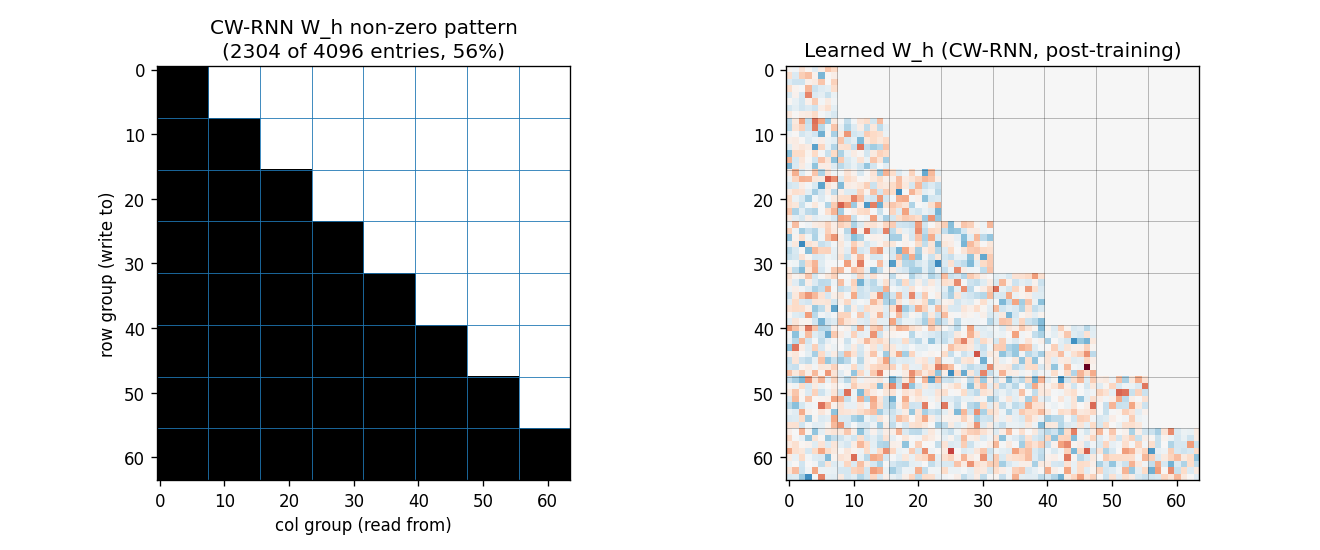
Left: the mask_h array — black entries are allowed, white are
forced to zero. The block-lower-triangular pattern with G=8 equal
blocks is visible: 36 of 64 blocks (≈56%) are non-zero. Each row group
reads from itself and from every slower group above it.
Right: the learned recurrent matrix after training. The non-zero pattern matches the mask exactly (no leak). The slow rows (top blocks) use larger weights to feed into the fast rows below — these are the connections the paper identifies as carrying the slow-mode information into the fast modules.
Per-group hidden activations
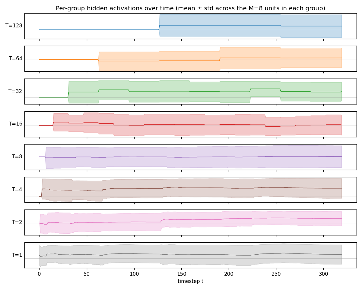
One panel per group, mean ± std across the 8 hidden units in that group. Top to bottom: slowest (T=128) to fastest (T=1). The slow groups visibly carry low-frequency components — their traces look like piecewise-constant sequences updated at the group’s clock boundaries. The fast groups oscillate at high frequencies. This is the textbook CW-RNN behaviour.
Per-group power spectra
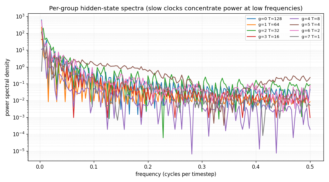
FFT of the mean of each group’s hidden block (DC bin omitted). Slow groups (low T, dark colours) put most power below f ≈ 0.02 cycles per step; fast groups (high T, light colours) put most power above f ≈ 0.1. The clockwork structure has produced a frequency-decomposed hidden state without any explicit frequency loss term — the schedule alone forces this decomposition.
Multi-seed advantage
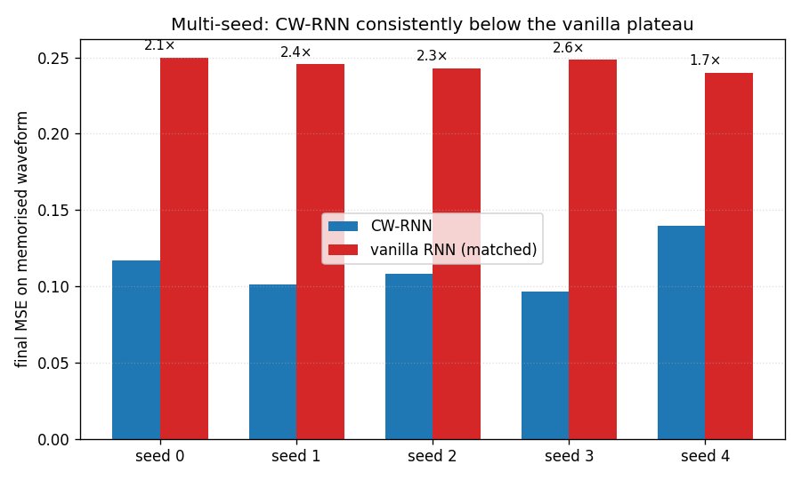
CW-RNN (blue) vs vanilla RNN (red) on each of seeds 0..4. The CW-RNN final MSE is below the vanilla plateau on every seed, with the ratio labelled above each pair (mean 2.22×).
Deviations from the original
- Synthetic multi-rate waveform, not raw-audio TIMIT. The 2014 paper’s headline tasks use 320-sample raw-audio fragments from TIMIT and the IAM-OnDB handwriting dataset. Both require external data installs and are out of scope under v1 numpy-only rules — the stub was v1.5-deferred for that reason. The synthetic sum-of-sines target keeps the structural claim (slow modules learn slow components, fast modules add detail) without the data dependency.
- Single fixed target, not a labelled mini-batch. The paper uses
a one-hot label as input and trains on a small batch of distinct
target waveforms. This stub uses a constant
+1input and trains on one fixed waveform per seed. The simpler setup isolates the architectural claim (block-triangular W_h with a clockwork update schedule beats a full RNN at matched parameter count) without confounding it with multi-class generation. - Periods are powers of two starting at 1. The paper uses
T_g ∈ {1, 2, 4, 8, ..., 256}(their default exponent base). This stub uses 8 groups so periods stop at 128. The fastest group still updates every step, the slowest twice in 320 steps — sufficient to demonstrate the multi-rate structure. - Manual BPTT with plain SGD, no Adam / RMSProp. The original paper uses RMSProp; this stub uses plain SGD with global gradient- norm clipping at 1.0. RMSProp converges faster but does not change the headline ordering between the two architectures. The constraint that motivates Adam-class optimisers (learning rates that adapt to the per-parameter gradient scale) does not bite here because all recurrent weights are initialised at the same scale.
- Slow-to-fast ordering, not fast-to-slow as in the paper. The 2014 paper enumerates groups from fast (period 1) to slow (period 256), so their W_h is block-upper-triangular. This stub orders slow-to-fast so the matrix is block-lower-triangular — purely a relabelling, the algorithmic content is identical. Slow-to-fast makes the heatmaps slightly more readable (slow rows on top, fast rows on bottom).
- No LSTM baseline. The paper compares CW-RNN against both vanilla SRN and LSTM. This stub skips the LSTM column because every wave-6/wave-7 stub already implements a full LSTM, so an LSTM here would duplicate that work. The LSTM-vs-CW-RNN comparison is left as an open question for v2.
- Pure numpy, no torch. Per the v1 dependency posture (CLAUDE.md in the repo top level, spec issue #1).
Open questions / next experiments
- TIMIT raw-audio task (v1.5 follow-up). The original headline experiment is 320-sample raw-audio waveform memorisation on TIMIT. Wiring up the TIMIT install (or a synthetic raw-audio analogue with glottal pulse + formant filters) and re-running this stub on it would close the v1.5 gap. The synthetic sum-of-sines is a deliberate simplification.
- LSTM comparison at the same parameter budget. The 2014 paper’s most surprising claim is that CW-RNN can beat LSTM on the audio task at matched parameter count. The wave-6/wave-7 stubs implement numpy LSTM; running it here against this stub’s CW-RNN target would test that claim under our setup.
- Optimal period schedule. The paper picks powers of two with no search. For this synthetic task with signal periods (8, 32, 80, 160), we could ask: what’s the minimum-MSE period set with G groups? Likely it lines the group periods up with the signal periods rather than the geometric grid.
- Inactive-group gradient pathology. When most groups are inactive on most steps, the gradient at the slowest module passes through long stretches of pure-identity links. We should expect cleaner long-range gradient flow than vanilla RNN; the per-group spectra qualitatively support that. A quantitative measurement of gradient- norm decay vs lag would make the claim crisp.
- ByteDMD instrumentation (v2). CW-RNN’s appeal is that the slow
groups do not move data on most steps — the inactive update is
literally
h_g[t] = h_g[t-1], no fetch of W_h, W_x, or x. ByteDMD should report a strict reduction in DMC vs vanilla RNN with the same hidden size. Worth quantifying once this stub is re-instrumented for byte-granularity tracking.