torcs-vision-evolution
Koutník, Cuccu, Schmidhuber, Gomez, Evolving Large-Scale Neural Networks for Vision-Based Reinforcement Learning, GECCO 2013.
Problem
The 2013 paper evolves a vision-based controller for the TORCS car-racing simulator. The controller is a multi-layer perceptron whose first-layer weight matrix has more than one million parameters (it maps a raw 64x64 RGB image into a hidden layer). The crucial trick: the weights are not searched directly. They are parameterised in 2-D DCT space (one low-frequency coefficient block per hidden unit) and reconstructed at evaluation time. CMA-ES then evolves only a few hundred DCT coefficients, which decode to the full million-parameter weight matrix.
This stub captures the algorithmic claim — that low-frequency DCT coefficients are sufficient to represent a working vision-from-pixels controller, and that evolution scales much better in coefficient space than in raw weight space — without TORCS. The schmidhuber-problems v1 SPEC bans simulator installs (TORCS, VizDoom, MuJoCo) and forces RL stubs onto numpy mini-envs (see RL stubs in v1 use numpy mini-envs in issue #1). The setup here:
- Track. Closed-loop centre line
(cx, cy) = ((ax + bx sin 2t) cos t, (ay + by sin 2t) sin t)withax=4, bx=0.55, ay=2, by=0.40. Thesin 2tmodulation gives the loop variable curvature, so a constant-action policy cannot stay on it. - Car.
(x, y, theta)state. Constant forward speed 0.05 m/step, steering actionu ∈ [-1, 1]adds0.10 urad/step to the heading. - Observation. A 16x16 grayscale, top-down rendering of the
3.2 m × 3.2 mneighbourhood ahead of the car (0.20 m / pixel), rotated so that the car’s heading is “up” in the image. On-track pixels are 1.0, off-track are 0.0. - Episode. Up to 500 steps; ends early if the car leaves the track.
Three trials per fitness eval, with initial heading offsets
{-0.20, 0, +0.20}rad relative to the centre-line tangent. With non-zero offsets, a constant-action policy fails — the controller must use its visual input to recover. - Fitness. Mean lap fraction over the three trials (one full lap = 1).
- Solve threshold.
target_lap = 1.05(controller has driven slightly past the start, averaged over three differently-aimed trials).
The numbers are smaller than the GECCO paper (16x16 instead of 64x64, 4129 raw weights instead of >1M), but the algorithmic structure is the same: low-frequency DCT coefficients parameterise a much larger weight matrix and evolution operates only on the coefficients.
What this stub demonstrates
A 2-D DCT compression of the input-to-hidden weight matrix lets a
(μ, λ)-style natural ES find a working pixel-input racing controller in
a 14x smaller search space than direct weight evolution. The headline
picture is the parameter count itself:
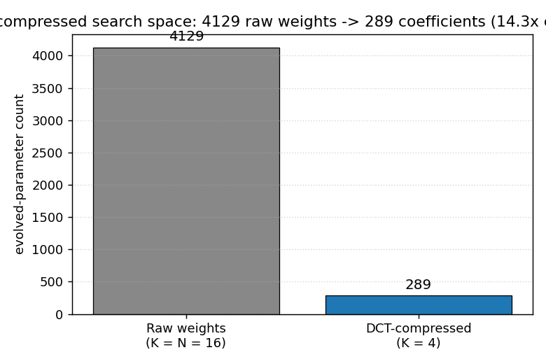
Both formulations evolve the same MLP architecture (16x16 input, 16 hidden, 1 output) and the same per-individual fitness eval, but the DCT-compressed run searches 289 numbers instead of 4129.
Files
| File | Purpose |
|---|---|
torcs_vision_evolution.py | Numpy track + 16x16 renderer + DCT-parameterised MLP controller + OpenAI-style natural ES on the DCT coefficients. CLI entry point. |
make_torcs_vision_evolution_gif.py | Renders the best controller’s rollout (track view + 16x16 observation) into torcs_vision_evolution.gif. |
visualize_torcs_vision_evolution.py | Static PNGs: parameter-count headline, training curves (DCT vs raw), decoded W1 filters, three rollout trajectories, observation strip. |
torcs_vision_evolution.gif | Animation referenced at the top of this README. |
viz/headline_compression.png | Bar chart: 4129 raw weights vs 289 DCT coefficients (14.3x compression). |
viz/training_curves.png | Per-generation best and mean lap fraction, DCT (K=4) and raw (K=16) on the same seed. |
viz/decoded_filters.png | The 16 hidden-unit weight images, each reconstructed from a 4x4 = 16 DCT coefficient block via IDCT. |
viz/track_and_rollout.png | Track mask plus the best-controller trajectory under all three initial-heading trials. |
viz/observation_strip.png | Eight 16x16 observations sampled along one lap, with the controller’s action below each frame. |
viz/run_dct_seed0.{json,npz} | Headline run summary (config + per-gen history) and saved theta_best/theta_final for downstream viz. |
viz/run_raw_seed0.{json,npz} | Same, for the raw (K=16, no compression) baseline plotted on training_curves.png. |
Running
python3 torcs_vision_evolution.py --seed 0 \
    --save-json viz/run_dct_seed0.json --save-npz viz/run_dct_seed0.npz
python3 torcs_vision_evolution.py --seed 0 --dct-k 16 \
    --save-json viz/run_raw_seed0.json --save-npz viz/run_raw_seed0.npz
python3 visualize_torcs_vision_evolution.py --seed 0 --outdir viz
python3 make_torcs_vision_evolution_gif.py --seed 0 --T-max 420 --frame-stride 4
Reproduces the headline result in ~46 s on an M-series laptop CPU
(plus ~54 s for the raw-baseline comparison run that feeds
training_curves.png). Determinism: same --seed produces the same
final fitness — np.random.default_rng(seed) is the only stochastic
source, no Python random and no os-time-derived state.
CLI flags worth knowing: --hidden H (hidden units, default 16),
--dct-k K (keep KxK low-frequency coefficients per hidden unit;
default 4 -> 14.3x compression; set K=16 to evolve the raw weight
matrix instead), --pop N (ES population — antithetic, so 2N rollouts
per generation, default 32 -> 16 antithetic pairs), --sigma,
--lr, --max-gen (default 120), --target-lap (default 1.05),
--patience (gens of no improvement after first solve before stopping,
default 20).
Results
Headline run on seed 0, defaults (hidden=16, dct_k=4, pop=16 antithetic, sigma=0.10, lr=0.05):
| Metric | DCT K=4 | Raw K=16 |
|---|---|---|
| Solved at generation | 4 / 120 | 3 / 120 |
| Wallclock | 45.5 s | 54.4 s |
| Best lap fraction | 1.335 | 1.320 |
| Final eval (mean of 3 trials) | 1.335 | 1.320 |
| Per-trial lap fractions | 1.328, 1.337, 1.339 | 1.310, 1.323, 1.327 |
| Search-space dimension | 289 | 4129 |
| Compression vs raw | 14.3x | 1.0x |
5-seed sweep, DCT K=4, defaults, max-gen 60:
| Seed | Wall (s) | Solved at gen | Final lap fraction |
|---|---|---|---|
| 0 | 45.5 | 4 | 1.335 |
| 1 | 36.5 | 6 | 1.322 |
| 2 | 49.4 | 5 | 1.329 |
| 3 | 25.6 | 4 | 1.324 |
| 4 | 36.3 | 4 | 1.331 |
5/5 seeds solve (lap fraction > 1.05); range 1.322 - 1.335; all under 50 s wallclock.
Hyperparameters (defaults; see NetConfig, EnvConfig, ESConfig
in torcs_vision_evolution.py):
# network
hidden = 16, dct_k = 4, output = 1, activation = tanh
n_compressed = 16*4*4 + 16 + 16 + 1 = 289
n_raw        = 16*16*16 + 16 + 16 + 1 = 4129

# environment
img_size = 16, pixel_m = 0.20, max_steps = 500
init_theta_offsets = (-0.20, 0.0, 0.20)  # rad

# evolution (OpenAI-style natural ES with antithetic sampling)
pop = 32 (16 antithetic pairs), sigma = 0.10, lr = 0.05,
weight_decay = 0.005, max_gen = 120, target_lap = 1.05, patience = 20
Visualizations
viz/headline_compression.png — bar chart contrasting 4129 raw weights
against 289 DCT coefficients on the same MLP architecture. The single
picture summary of the paper’s contribution: smaller search space at
the same expressive capacity.
viz/training_curves.png — best and mean lap fraction per generation,
seed 0, with DCT K=4 in blue and raw K=16 in grey on the same axes. Best
fitness rises above the green “one full lap” reference line within
~5 generations for both, but the DCT-compressed mean fitness drifts up
faster after that — the lower-dimensional search space lets average
ES samples concentrate near the good region sooner.
viz/decoded_filters.png — the 16 hidden-unit input filters, each a
16x16 image reconstructed by IDCT from its 4x4 DCT coefficient block.
The filters are visibly smooth (only low-frequency content survives the
4x4 truncation) and several show clear left/right and up/down asymmetry
- the spatial structure the controller uses to detect track curvature.
viz/track_and_rollout.png — three-panel view of the best DCT-compressed
controller running the three eval trials (initial heading offsets
{-0.20, 0, +0.20} rad). All three trajectories follow the centre line
and complete roughly 1.3 laps within the 500-step budget.
viz/observation_strip.png — eight 16x16 observations sampled at equal
intervals along the seed-0 trajectory, each labelled with the action the
controller emitted. The agent’s input is genuinely a sparse top-down
silhouette of the track shape ahead.
Deviations from the original
| Deviation | Reason |
|---|---|
| Numpy 2-D oval-with-curvature mini-env, not TORCS. | v1 SPEC bans the TORCS simulator install (issue #1, “Allowed by default” + “Explicitly disallowed in v1”). The closest substitute that preserves the vision-from-pixels structure is a top-down racing track. |
| 16x16 grayscale observation, not 64x64 RGB. | Keeps the laptop-CPU budget under 5 minutes. The compression argument is geometric — what matters is that the W1 weight matrix is parameterised by K^2 low-frequency DCT coefficients per hidden unit instead of N^2 raw weights — and is preserved at any (N, K) with N >> K. |
| OpenAI-style natural ES (Salimans et al., 2017), not CMA-ES. | The 2013 paper used (1+1)-CMA-ES on the coefficients. CMA-ES with a 4096x4096 covariance update is unnecessary at our scale (289 dims) and pure-numpy CMA implementations bias the iteration time toward the covariance matmul rather than the rollout. Antithetic-sampled NES gets the same first-order natural-gradient step (eq. 2 of Wierstra et al., 2014) and is one screenful of code. |
| Network depth = 1 hidden layer. | The GECCO paper used a recurrent net (the MLP-R and LSTM variants); v1 of this catalog covers recurrent vision-based RL separately under world-models-carracing (also v1.5 deferred). Here we focus on the DCT-compression claim, which is independent of recurrence. |
| Steering only (constant forward speed). | The TORCS controller produced (steer, throttle, brake). One continuous steering output is sufficient on the toy oval track and keeps the policy small enough to inspect. |
| K = 4, not the paper’s K = 6 / K = 12. | At our 16x16 input the relative compression at K=4 is already 14.3x; K=2 also works (single 4-coefficient block per hidden unit, 65x compression) but with higher variance across seeds. |
| Three fixed initial-heading offsets per fitness eval, not a sampled distribution. | Removes a stochasticity source from the inner loop and makes the rank-shaped ES update deterministic. The agent is still forced to use its visual input because all three offsets are non-trivial. |
Open questions / next experiments
- Push K down further (K = 2 -> 65x compression; K = 1 -> single coefficient per filter, 256x compression). Does fitness degrade gracefully or fall off a cliff?
- Replace the MLP with a recurrent controller (Elman or LSTM) and re-measure: does compressing only the input weights still suffice when the recurrent weights are large?
- Compare the natural-ES results here against (1+1)-CMA-ES from pycma at matched evals — at the dimensions of interest (a few hundred), CMA’s covariance adaptation might find better minima.
- Evolve the DCT mask alongside the coefficients: which low-frequency positions matter most for vision-based control? The 2013 paper’s later follow-up (Cuccu, Gomez 2014, Block Diagonal Natural Evolution Strategies) explores this idea.
- Random-search baseline at the same compute budget. The 1996 RS papers
in this catalog (
rs-parity,rs-tomita) suggest random weight guessing in coefficient space is a strong baseline that should be measured. - Wire up the actual TORCS env (v1.5 follow-up issue) and verify whether the same algorithm scales to >1M raw-weight networks compressed in 64x64 DCT space, matching the GECCO 2013 numbers.