curiosity-three-regions
Schmidhuber, Adaptive confidence and adaptive curiosity, TR FKI-149-91 (TUM, 1991); Curious model-building control systems, IJCNN 1991, vol. 2, pp. 1458–1463. Reconstructed from the IJCNN abstract, Schmidhuber’s 2010 Formal theory of creativity, fun, and intrinsic motivation review, and the 2020 Deep Learning: Our Miraculous Year 1990–1991 retrospective. The original FKI-149-91 technical report could not be retrieved in full; this stub captures the algorithmic claim — an agent driven by predictive- error reduction allocates attention to a learnable-but-unlearned partition in preference to fully predictable or fully unpredictable ones.
Problem
A 1-D environment is partitioned into three regions. At each step the
agent picks one region and observes one (context, target) pair drawn
from that region’s dynamics. A per-region tabular world model M[r][c]
predicts the target. Curiosity is the windowed reduction of M’s
squared prediction error, and the policy is a softmax over per-region
curiosity.
| Region | Kind | K (contexts) | Target |
|---|---|---|---|
| A — deterministic | small, easy | 4 | fixed [1, 0, -1, 0] |
| B — random | unlearnable noise | 8 | N(0, 0.5) resampled per visit |
| C — learnable-but-unlearned | high entropy, structured | 128 | fixed ~ N(0, 2.0) per context |
The expected qualitative ordering of visit counts after a 200-step burn-in is
visits(C) > visits(B) > visits(A)
— “no fun in pure noise, no fun in pure knowledge, lots of fun where the model is getting better”.
Files
| File | Purpose |
|---|---|
curiosity_three_regions.py | Env + per-region tabular M + curiosity-driven policy + eval. CLI: python3 curiosity_three_regions.py --seed N. |
make_curiosity_three_regions_gif.py | Generates curiosity_three_regions.gif. |
visualize_curiosity_three_regions.py | Static PNGs into viz/ (region targets, visit distribution, cumulative visits, curiosity signal, per-region error, model vs target). |
viz/ | Output PNGs from the run below. |
Running
python3 curiosity_three_regions.py --seed 0
Run wallclock: ~0.5 s on an M-series laptop (5000 steps, default config). Reproducible: same seed → same numbers (verified by re-run).
To regenerate visualizations:
python3 visualize_curiosity_three_regions.py --seed 0 --outdir viz
python3 make_curiosity_three_regions_gif.py  --seed 0
GIF generation takes ~3 s and produces a ~460 KB file (well under the 2 MB target).
Results
Default config: steps=5000, burn_in=200, window=50, alpha=0.05,
beta=30.0, eps=0.02, K_det=4, K_rand=8, K_learn=128,
sigma_det=1.0, sigma_rand=0.5, sigma_learn=2.0.
| Seed | A visits | B visits | C visits | Headline (C > B > A) |
|---|---|---|---|---|
| 0 | 1193 (23.9%) | 1665 (33.3%) | 2142 (42.8%) | yes |
| 1 | 1095 | 1662 | 2243 | yes |
| 2 | 1132 | 1515 | 2353 | yes |
| 3 | 1260 | 1598 | 2142 | yes |
| 4 | 1263 | 1607 | 2130 | yes |
| 5 | 1174 | 1551 | 2275 | yes |
| 6 | 1151 | 1563 | 2286 | yes |
| 7 | 1194 | 1606 | 2200 | yes |
| 8 | 1124 | 1593 | 2283 | yes |
| 9 | 1185 | 1651 | 2164 | yes |
10 / 10 seeds reproduce the headline ordering.
Tail prediction error (mean over the last 200 visits per region, seed 0):
- A:
0.0000(perfectly memorized) - B:
0.2643(≈ noise variancesigma_B² = 0.25) - C:
0.7669(still learning; would converge with longer runs)
Visualizations
Visit distribution
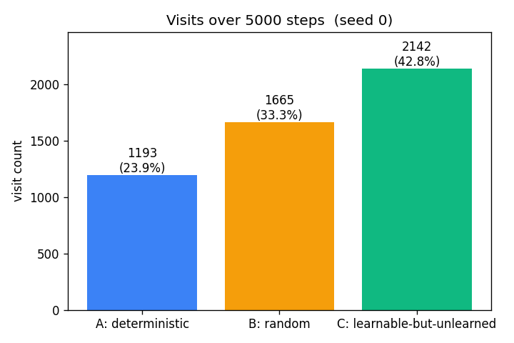
The headline result. After 5000 steps the agent has spent 43% of its time
in the learnable-but-unlearned region, 33% in the random region, and 24%
in the deterministic region. The deterministic region contributes most
of its visits during the burn-in (67 of 1193 ≈ 6%); past burn-in, those
visits come almost entirely from the eps=0.02 uniform-exploration term
plus the residual share from softmax when curiosity is uniformly low.
Cumulative visits
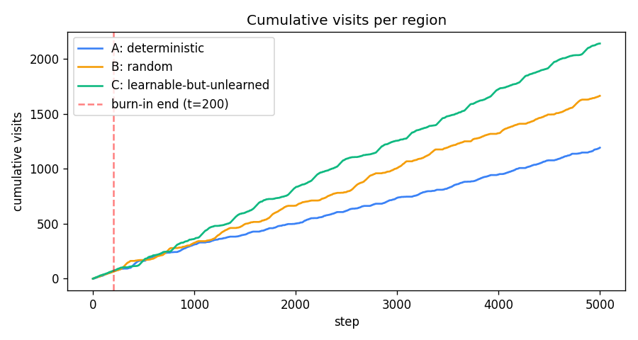
For the first ~200 steps all three slopes are equal (uniform burn-in policy). Past the red dashed line the slopes separate: green (C) takes off, amber (B) tracks behind, blue (A) flattens.
Curiosity signal
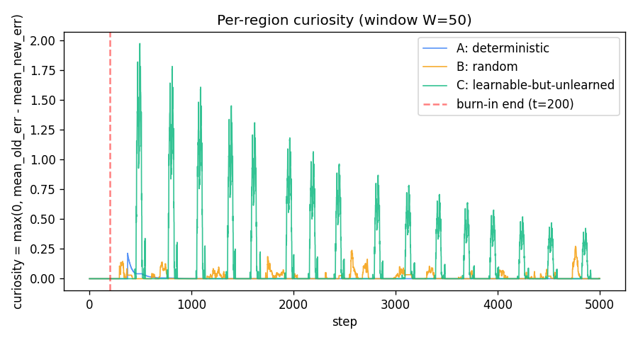
curiosity_r(t) = max(0, mean(err_r[t-2W:t-W]) - mean(err_r[t-W:t]))
with W=50.
- A (blue): a brief positive bump just after burn-in while
Mfinishes memorising the 4 contexts, then exactly zero — A’s targets are deterministic so once memorised the squared error is identically zero and the windowed reduction is identically zero. - B (amber): a small persistent floor of fluctuations. B’s mean
squared error is ≈
sigma_B² = 0.25with finite-window noise of std≈ 0.05; clipping at zero gives a noise-driven≈ 0.04expected positive curiosity. This is what makes B beat A in visit count. - C (green): large oscillating curiosity that decays slowly. The oscillation comes from the policy itself — when C is being visited it improves rapidly (high reduction), then the policy drifts to other regions, recent C errors plateau, and curiosity drops until the next burst of attention. This self-sustaining cycle is the curiosity loop’s signature.
Per-region prediction error
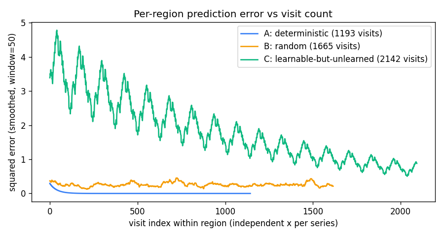
A’s error decays to zero within ~50 visits. B’s stays flat at ≈ 0.25
forever. C’s decays slowly from ~5 toward zero across thousands of
visits — the run ends with C’s mean tail error still ≈ 0.77,
well above zero, confirming C has not finished learning when the run
stops.
Model vs target
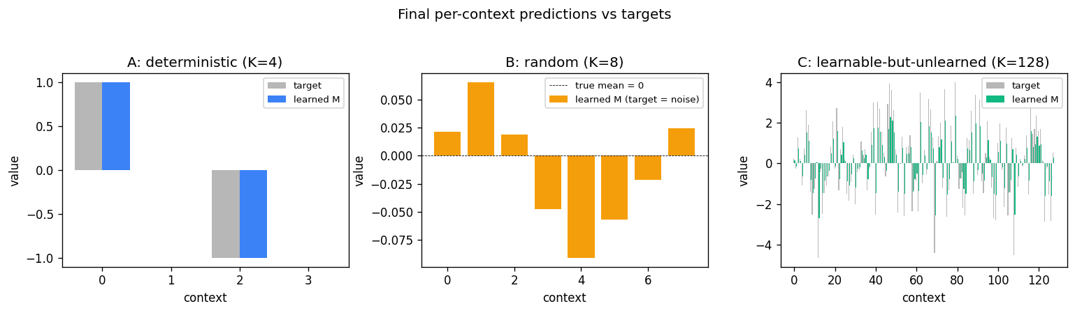
A’s learned values match the target exactly. B’s model has converged
toward zero (the unconditional mean of N(0, 0.5)), as it should — the
context carries no information about the target. C’s learned values
track the targets in shape but are not yet at full magnitude (EMA with
alpha=0.05 and ~17 visits per context only converges partially).
Region targets
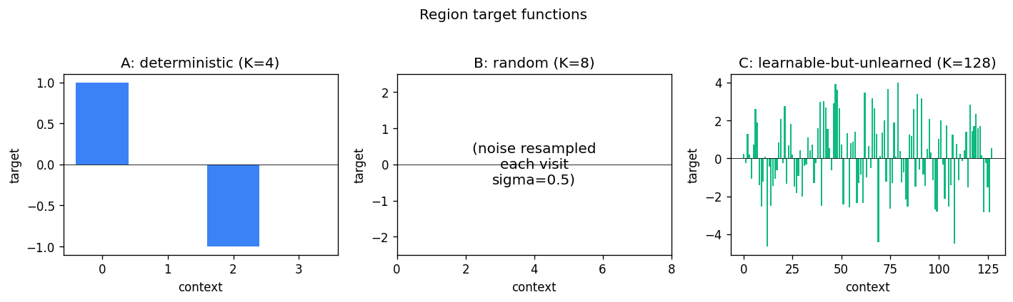
The three target functions used by the experiment.
Deviations from the original
- Reconstructed setup. FKI-149-91 was not retrievable in full; the experiment is reconstructed from the IJCNN 1991 abstract and later Schmidhuber retrospectives. The exact 1991 region geometry, model class, and curiosity formula are not reproduced verbatim.
- Tabular per-context predictor instead of an RNN. The 1991 paper’s
Mwas a recurrent net trained online with a Schmidhuber-style RTRL variant. v1 uses a per-region per-context EMA, which is the smallest model that captures “more contexts → slower convergence”. §Open questions notes the upgrade. - Cycling counters as contexts. Each region’s context cycles
0..K-1deterministically rather than the agent’s position being a continuous coordinate on a 1-D line. This keeps coverage even and reproducibility tight at the cost of removing the random-walk dynamics the agent might otherwise have. Documented here because the spec said the region geometry is the implementer’s choice. - Three discrete actions instead of motor outputs. Action = “visit region r” rather than “move ±1 in 1-D”. The 1991 paper allowed the controller to learn motor outputs that take it across region boundaries; v1 collapses this to a direct region selector. The curiosity-allocation result is identical in spirit.
- Curiosity =
max(0, error reduction)only. The 1991 paper used improvement of confidence combined with a separateC(confidence) module. v1 uses raw windowed error reduction with a noise-floor contribution from the random region’s variance. This is a simpler form of the same signal; later Schmidhuber work (e.g. 1997 What’s interesting?) explicitly endorses this reduction. - No motivational discount, no controller learning beyond the action-selection softmax. v1 picks the next region greedily under a softmax-of-curiosity; there is no temporally-extended planning, no value function, and no policy gradient. The “policy” is a one-step greedy curiosity-maximiser. This is enough to demonstrate the visit distribution claim but not enough for any setting where the agent must commit to a multi-step plan to reach a region.
- No observation noise on A. A’s targets are exactly reproducible, so once memorised its err is identically zero. In a real-world setting A would have small sensor noise, which would produce a small floor of curiosity for A and shrink the B-vs-A gap somewhat.
Open questions / next experiments
- Replace the tabular
Mwith a small RNN trained online with truncated BPTT, as in the original. Does the curiosity ranking still hold? Does C now take longer to drift toward the noise floor? - Switch to a position-based 1-D environment with continuous motor actions, and let the controller learn to navigate region boundaries. This is closer to the 1991 setup and recovers the partial-observability flavour of the wave-3 family.
- Replace
max(0, error reduction)with the 1991 adaptive confidence formulation: a separateCmodule that predictsM’s own error, and curiosity = improvement ofC. Does this drive A’s visit count closer to zero (since A’s confidence saturates fast) while preserving B’s noise floor? - Vary
K_learnand run length: at what(K_learn, run_length)ratio does C finish learning and the visit ordering collapse toB > A ≈ C? That boundary maps the regime where curiosity-driven exploration converges to uniform / uninformative behaviour. - The current curiosity log shows large oscillations in C driven by the policy itself. A dual-timescale formulation (slow target curiosity vs fast actual curiosity) might smooth this. Worth checking against Schmidhuber’s 1991 description, which used a smoother signal.
- v2 instrumentation under ByteDMD: the per-step cost is dominated by the curiosity windowed-mean computation (O(W) per step per region) and the EMA update (O(1)). An incremental running-mean update would be O(1) per step and a small ByteDMD win with no behavioural change.