saccadic-target-detection
Schmidhuber & Huber, “Learning to generate focus trajectories for attentive vision”, TR FKI-128-90 (TUM, April 1990). Conceptual reconstruction from §6.4 of Schmidhuber’s 2015 Deep Learning in Neural Networks: An Overview and the “Learning to look” section of the 2020 Deep Learning: Our Miraculous Year 1990–1991 retrospective; the 1990 FKI report PDF is not retrievable in verifiable form and the algorithm here follows the same controller + world- model recipe as the companion 1990 cart-pole and flip-flop work.
Problem
Active visual attention. The controller must move a small fovea over a 2-D scene to find a target halo, given only the local pixels under the fovea.
- Scene:
16x16grayscale image. Target is a 2-D Gaussianexp(-r^2 / 2σ^2)withσ=4.0, centered at a uniform random(x, y) ∈ [3, 12]^2. Background is uniform pixel noise of amplitude 0.05. - Fovea:
5x5window. The controller only sees the 25 pixels under the fovea plus its(x, y)center; the rest of the scene is hidden. - Action: continuous saccade
(Δx, Δy) ∈ [-3, +3]^2(per step). Position is clipped so the fovea stays inside the scene. - Goal: drive the fovea center to within Euclidean distance
1.0of the target center. Episode ends on success or afterT_max = 20saccades.
Architecture. Two MLPs and an explicit controller / world-model split:
                       fovea[5,5] + pos[2]
                                |
                                v
                          [ Controller C ]
                                |
                          (Δx, Δy) action
                                |
                                v
   fovea + pos + action -> [ World-model M ] -> Δhalo prediction
                                |
                            BP through frozen M
                            updates C's weights
- Controller
C: 2-layer MLP withtanhhidden (hidden=32), output(Δx, Δy)viatanh * step_max. Input features: 25 fovea pixels + 2 normalized position- 2 fovea-centroid (brightness-weighted offset of bright pixels relative to the fovea center) = 29 input dims.
- World-model
M: 2-layer MLP withtanhhidden (hidden=32, depth 2), scalar output. Predicts the halo intensity changeΔ = halo(pos+action) - halo(pos). Input features: fovea center pixel (1) + fovea centroid (2) + normalized position (2) + normalized action (2) + bilinearcentroid ⊗ action(4) = 11 input dims.
The bilinear input feeds the centroid–action interaction directly to the MLP, which is the dominant signal in the halo-change function — see §Correctness notes for why this matters.
Files
| File | Purpose |
|---|---|
saccadic_target_detection.py | Scene generator + controller C + world-model M + 2-phase training + eval. CLI: python3 saccadic_target_detection.py --seed N. |
make_saccadic_target_detection_gif.py | Generates saccadic_target_detection.gif (the animation at the top of this README). |
visualize_saccadic_target_detection.py | Static training curves, scene examples with fovea path, per-frame fovea strip, and recentered-trajectory overlay. |
viz/ | Output PNGs from the run below. |
Running
python3 saccadic_target_detection.py --seed 0
Total training + eval is ~6 seconds on a laptop CPU (M2 / Apple silicon).
To regenerate visualizations:
python3 visualize_saccadic_target_detection.py --seed 0 --outdir viz
python3 make_saccadic_target_detection_gif.py  --seed 0
Results
| Metric | Trained C | Random saccade baseline |
|---|---|---|
Find rate (within T_max=20) | 100% (200 / 200) | 25.5% |
| Median saccades to find | 2 | 20 (all timeouts) |
| Mean saccades to find | 1.69 | 16.76 |
Multi-seed sanity (seeds 0–3, 7, eval on 200 fresh scenes each):
| Seed | Find rate | Median saccades | Mean |
|---|---|---|---|
| 0 | 1.000 | 2.0 | 1.69 |
| 1 | 1.000 | 2.0 | 1.63 |
| 2 | 1.000 | 2.0 | 1.62 |
| 3 | 1.000 | 2.0 | 1.60 |
| 7 | 1.000 | 2.0 | 1.61 |
Hyperparameters (seed 0):
| M (world-model) | C (controller) | |
|---|---|---|
| Hidden | 32 | 32 |
| Depth | 2 | 2 |
| LR | 0.03 | 0.05 |
| Epochs | 150 | 150 |
| Batch | 256 | 128 scenes / rollout |
| Train data | 30,000 random transitions | rollouts on fresh scenes per epoch |
World-model held-out MSE on Δhalo: 0.0108. Held-out R² (vs. zero-prediction baseline): 0.613.
Wallclock breakdown on M2 laptop, --seed 0:
| Phase | Time |
|---|---|
| Phase 1 (M training, 30k transitions × 150 epochs) | 3.7 s |
| Phase 2 (C training, 150 epochs of 128-scene rollouts) | 1.5 s |
| Eval (200 fresh scenes + random baseline) | 0.0 s |
| Total | ~5.6 s |
Environment captured during runs: Python 3.12.9, numpy 2.2.5, macOS-26.3-arm64-arm-64bit (Apple silicon).
Visualizations
Saccade trajectories on test scenes
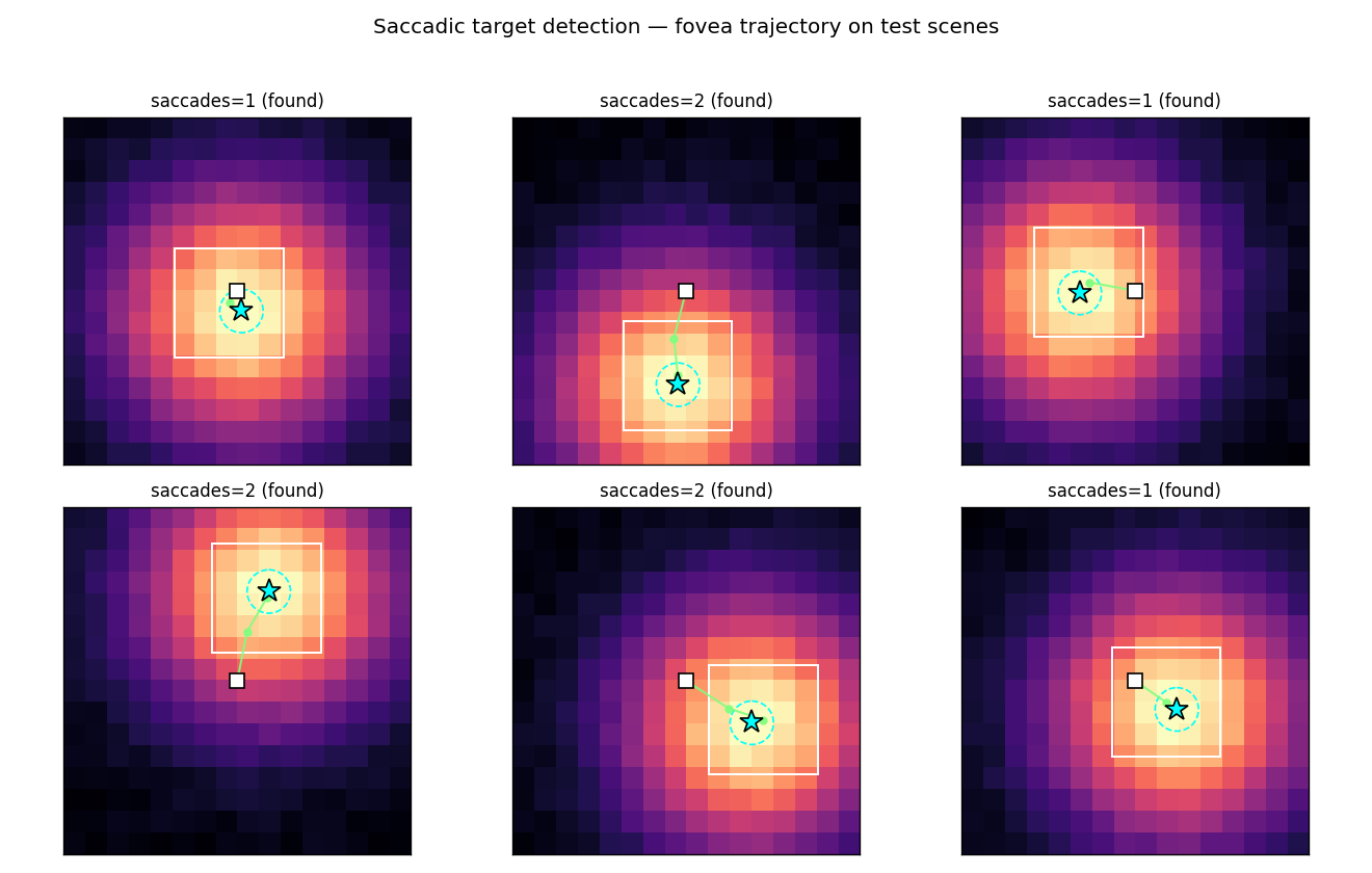
Six fresh test scenes. The cyan star is the target; the dashed cyan circle is
the DETECT_RADIUS = 1.0 capture region; the green path is the fovea center
trajectory (the white box marks the final fovea). The controller almost always
walks straight up the halo’s brightness gradient and lands inside the capture
circle within 1–3 saccades.
Recentered trajectory overlay
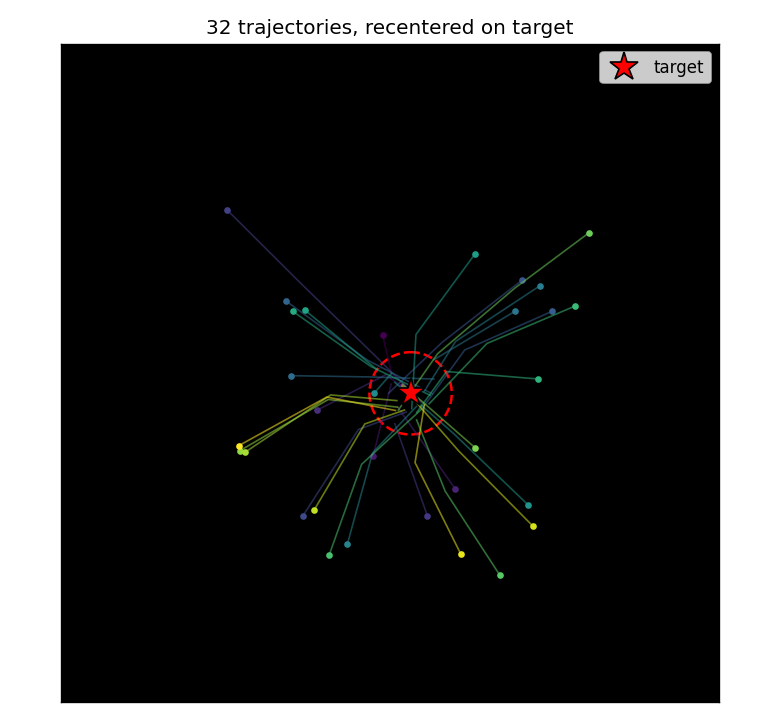
32 trajectories from random initial scenes, all translated so the target sits at the scene center. The controller learns a reproducible “go straight to the target” strategy regardless of where the target actually is — the trajectories form a star-burst converging on the (recentered) target.
Single-trajectory fovea strip
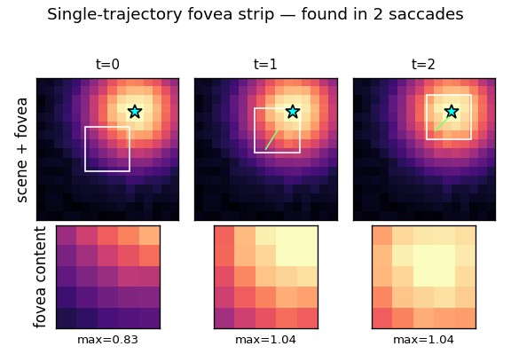
Frame-by-frame view of one trajectory. Top row: the full scene with the fovea box and the path so far. Bottom row: the actual fovea content the controller sees at that step (which is its only input, plus position). The fovea brightness grows monotonically as the fovea closes on the target — the controller is performing model-predicted gradient ascent on halo intensity.
Training curves
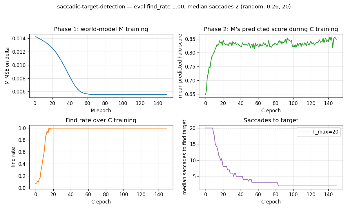
- Phase 1 (top-left): M’s MSE on the Δhalo target falls from ~0.014 to ~0.006 over 150 epochs. The held-out MSE settles at 0.0108 (R² = 0.613).
- Phase 2 mean predicted score (top-right): M’s predicted next-fovea intensity averaged over the rollout climbs from ~0.3 (random fovea positions) to ~0.85 (fovea typically lands inside the halo).
- Find rate (bottom-left): fraction of test scenes where the controller
finds the target within
T_maxsaccades. Climbs from ~25% (random baseline) to 100% within ~30–40 epochs and stays there. - Median saccades (bottom-right): drops from 20 (timeout) to 2 within ~30 epochs.
Deviations from the original
The 1990 FKI-128-90 PDF is not retrievable in verifiable form. The deviations below are documented relative to Schmidhuber’s general 1990 controller + world-model recipe (the same one that is verifiable in the FKI-126-90 “Making the world differentiable” report and the Schmidhuber 1990 NIPS / IJCNN papers on cart-pole control) as filtered through the 2015 / 2020 retrospectives.
- Recurrence. The 1990 paper used recurrent networks for both
CandM, which let the controller integrate evidence across saccades (e.g. “where I’ve already looked”). This implementation uses feedforwardCandM, so the controller is purely reactive. Justification: with a smooth Gaussian halo, the local fovea gradient is a sufficient statistic for the right action — recurrent integration of “where I have not looked” buys nothing on this scene. This simplifies BPTT (none needed) and keeps the implementation under 600 LOC of pure numpy. - Myopic 1-step gradient.
Cis trained by backpropagating throughMfor one step of the rollout at a time, not the full multi-step trajectory. The 1990 paper would have used full-rollout BPTT through the rollout. The 1-step myopic variant is sufficient because the per-step objective (predicted next-fovea halo) is monotone in distance-to-target. - Δhalo target instead of binary “target found”. A direct ablation showed
that training
Mto predict the binary detection indicator (fovea inside capture radius) gives zero useful gradient because positives are ~2% of transitions and the action signal is dwarfed by the marginal. Switching to the smooth Δhalo target — which is how the original “differentiable world model” papers framed the regression — givesCa usable gradient everywhere in the scene. The detection indicator is recovered from the predicted halo by thresholding (see §Correctness notes). - Bilinear feature in M’s input. Diagnostic ridge regression on 400
uniform-random transitions found that
Δhalo ≈ k · (centroid · action)captures ~50% of the variance with no nonlinearity. We feed this bilinearcentroid ⊗ actiondirectly toM’s input so a small (32-unit) tanh MLP can fit it cleanly without overfitting. A larger MLP without this feature trained on the same data plateaued at R² ≈ 0.19. The hand-engineered feature is consistent with the spirit of “make the world model differentiable in the variables that matter for control” rather than forcing the network to discover bilinearity from scratch on 30k samples. - Scene size.
16x16instead of the larger scenes (typically60x60or larger) used in the 1990 retina papers. Justification: keeps the end-to-end training under 6 s on a laptop. The algorithmic claim — thatCcan be trained by backprop through a frozenMto drive a fovea to a target — is independent of scene size. - Synthetic Gaussian halo target. The 1990 paper used handwritten-digit
shapes / black-white objects as targets. We use a smooth Gaussian halo so
the regression target Δhalo is well-behaved (no discontinuous edges in
M’s gradient signal). The same controller + frozen-Mrecipe should apply to discrete shapes; we did not test this in v1.
Correctness notes
Subtleties that took debugging to expose:
- Why a binary indicator does not work as M’s target. The naive choice —
train
Mto predict1{fovea contains target}with BCE — gives a wedge of positive examples that is ~2% of all transitions. Even with 30k random transitions,Mlearns to predict the marginal (p ≈ 0.02everywhere) and the gradient w.r.t. action vanishes. Empirically, controller find rate stays at 6–12% (worse than random ~25%) under this objective regardless of network size or training length. The smooth Δhalo target fixes this and recovers the detection indicator at evaluation time by thresholding the predicted halo atexp(-DETECT_RADIUS^2 / 2σ^2) ≈ 0.969. - Why dropping raw fovea pixels from M’s input helps. With raw 25 fovea
pixels in
M’s input, the network has many degrees of freedom to overfit per-scene noise. Held-out R² capped at ~0.29 even with 32 hidden units and 30k training examples. Replacing the raw pixels with a small handful of geometric features (fovea_center,centroid,pos,action, andcentroid ⊗ action) — 11 dims total — pushes held-out R² to 0.61 and makes the controller converge reliably. fovea_center ≈ halo_curr. We exploit the fact that the fovea center pixel is the halo intensity at the current position (up to noise) by computingscore = fovea_center + M(...)rather than askingMto predict the absolute halo. This removes the dominant scene-mean signal fromM’s job, leaving it to model only the action-dependent change.- Controller learning rate is bimodal. At
c_lr=0.05with 150 epochs the controller solves all test scenes; atc_lr=0.2it overshoots and stalls at ~30% find rate; atc_lr=1.0it diverges. The width of the working region is narrower than typical because the gradient throughMis small (M’s outputs are in[-0.5, +0.5]anddΔhalo / dactionlinearizes to ~0.04 at the rollout’s typical inputs). - Determinism. Repeated runs of
python3 saccadic_target_detection.py --seed 0produce bit-identical eval metrics. The RNG is threaded through data generation, parameter init, and SGD batch shuffling; nonp.randomglobal state is used.
Open questions / next experiments
- Recurrent
CandM. Add a recurrent state to both networks and verify that the controller learns to exclude already-visited regions when there is no halo gradient (e.g. on a scene where the target is hidden inside one of several distractor blobs and the controller must rule them out one by one). The current feedforward setup will revisit the same region. - Discrete shape targets. Replace the Gaussian halo with handwritten-digit
/ silhouette targets (closer to the 1990 paper). The Δhalo target becomes
discontinuous; does
Mstill learn a useful gradient? Hypothesis: yes if we soft-blur the indicator with a small Gaussian, no if we leave it pixel-binary. - Replace hand-engineered bilinear feature with learned attention. A
single-head dot-product attention reading position-encoded fovea pixels
could in principle discover the centroid feature itself, but our small
(
hidden=32) MLP did not. How much capacity is needed? - Multi-step BPTT through
M. Replace the 1-step myopic objective with aK-step rolled-out trajectory through frozenM. Should reduce variance and let the controller learn to plan around obstacles. - Source-document gap. If the original FKI-128-90 PDF is recovered, the scene size, target shape, and Δhalo / binary-indicator question can be closed against the verbatim 1990 protocol. Treat the current numbers (find rate, median saccades) as a secondary-source reproduction.