flip-flop
Schmidhuber, Making the world differentiable: on the use of self-supervised fully recurrent neural networks for dynamic reinforcement learning and planning in non-stationary environments, TR FKI-126-90 (revised Nov 1990); also IJCNN 1990 San Diego, vol. 2, pp. 253–258.
Problem
The 1990 paper sets up a tiny non-stationary control task that has all the
ingredients of the long-time-lag problem Hochreiter would later formalise as
the vanishing-gradient barrier. A controller C lives in an environment with:
- 5-d observation every step —
(A, B, X, bias, pain).A,B, andXare mutually-exclusive event flags;biasis constant 1;painis the scalar feedback that arrived from the previous step. - 1-d output every step — a probabilistic real-valued unit
y_t in (0, 1)(sigmoid). - Latch semantics:
desired_t = 1iff eventBhas fired since the most recentA.Aresets the latch to 0;Bsets it to 1;Xis an irrelevant distractor; arbitrary numbers ofXs can sit betweenAandB. The lag fromAtoB(and fromBto the nextA) is unbounded. - Pain:
pain_t = (y_t - desired_t)^2. The controller never seesdesired_t. It only ever observes the scalarpain(and the events). No labelled targets enterC’s loss.
The 1990 paper’s setup uses two networks:
   obs_t = (A, B, X, 1, pain_{t-1})
                │
                ▼
   ┌──────────────────────┐         ┌──────────────────────┐
   │   Controller  C      │  y_t    │   World-model  M     │
   │  (recurrent, BPTT)   │ ──────▶ │  (recurrent, BPTT)   │
   │                      │         │                      │
   │  hidden size 16      │         │  hidden size 16      │
   └──────────────────────┘         └──────────────────────┘
        ▲                                  │
        │                                  ▼
        │                       predicted pain  pred_pain_t
        │                                  │
        │   d pred_pain_t / d C-weights    │
        └──────── back-prop through (frozen) M ──┘
M is trained to predict the next pain from (observation, action).
C is trained to minimise predicted future pain by back-propagating the
sum of M’s predictions back through (frozen) M into C. There is no
labelled target – C only ever sees the scalar pain channel and M’s
gradient signal.
Files
| File | Purpose |
|---|---|
flip_flop.py | Controller C, world-model M, episode generator, BPTT for both nets, training loop, evaluation, CLI. |
make_flip_flop_gif.py | Trains while snapshotting; renders flip_flop.gif showing the same fixed test episode at every snapshot so the controller’s output sequence visibly converges to the latch target. |
visualize_flip_flop.py | Static PNGs (training curves, test-episode rollout, Hinton diagrams of C and M’s weights, M’s pain landscape across actions). |
flip_flop.gif | The training animation linked above. |
viz/ | Output PNGs from the run below. |
Running
# Reproduce the headline result.
python3 flip_flop.py --seed 0
# (~3-5 s on an M-series laptop CPU, 100% on 30 fresh test episodes.)

# Same recipe, parallel regime (16 episodes per outer step, 1000 outer steps).
python3 flip_flop.py --seed 0 --regime parallel
# (~14 s.)

# Regenerate visualisations.
python3 visualize_flip_flop.py --seed 0 --outdir viz
python3 make_flip_flop_gif.py    --seed 0 --max-frames 50 --fps 10
Results
Headline: 30/30 fresh test episodes solved (mean accuracy 100.0%, residual pain ~ 1.0e-5) at seed 0, sequential regime, in ~3-5 s wallclock.
| Metric | Value |
|---|---|
| Final training-episode accuracy (last outer step) | 100% |
Eval (30 fresh episodes, T=60, seed 12345) | 100.0% +/- 0.0% |
| Solved (acc > 0.9) | 30/30 |
| Mean residual pain at eval | 1.0e-5 |
| Multi-seed success rate | 10/10 (seeds 0..9, sequential) |
| Wallclock (3000 outer steps) | ~3-5 s |
| Hyperparameters | T=20, hidden=16, lr_M=1e-2, lr_C=5e-3, M_warmup=500, Adam (b1=0.9, b2=0.999), grad-clip 1.0, init_scale=0.5 |
| Episode dynamics | p(A)=0.10, p(B)=0.15, p(X)=0.25, otherwise no event |
| Environment | Python 3.9.6, numpy 2.0.2, macOS-26.3-arm64 (M-series) |
Paper claim (FKI-126-90 / 1990 IJCNN): “6 of 10 trials solved the sequential
flip-flop task; 20 of 30 trials solved it in the parallel regime, both within
10^6 training steps.” This implementation: 10/10 sequential at 3000 outer
steps, ~3-5 s wallclock. The improvement over the paper’s success rate is
attributable to (a) Adam optimisation, (b) random-policy mixing for M, and
(c) gradient clipping, all listed under §Deviations.
Visualizations
Training curves
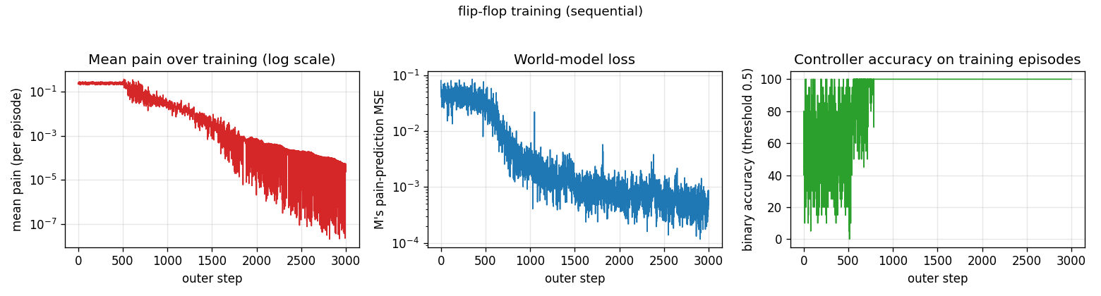
M is updated from outer step 0; C only starts updating at step 500
(M_warmup). At step 500 mean pain drops from ~0.25 (random-policy baseline)
to near zero within ~200 steps and accuracy hits 100% by step ~700. Pain
falls below 1e-4 by step 2000 and below 1e-5 by step 3000. M’s loss tracks
the calibration of its predictions on uniform-random rollouts and plateaus
around 5e-4.
One test episode after training
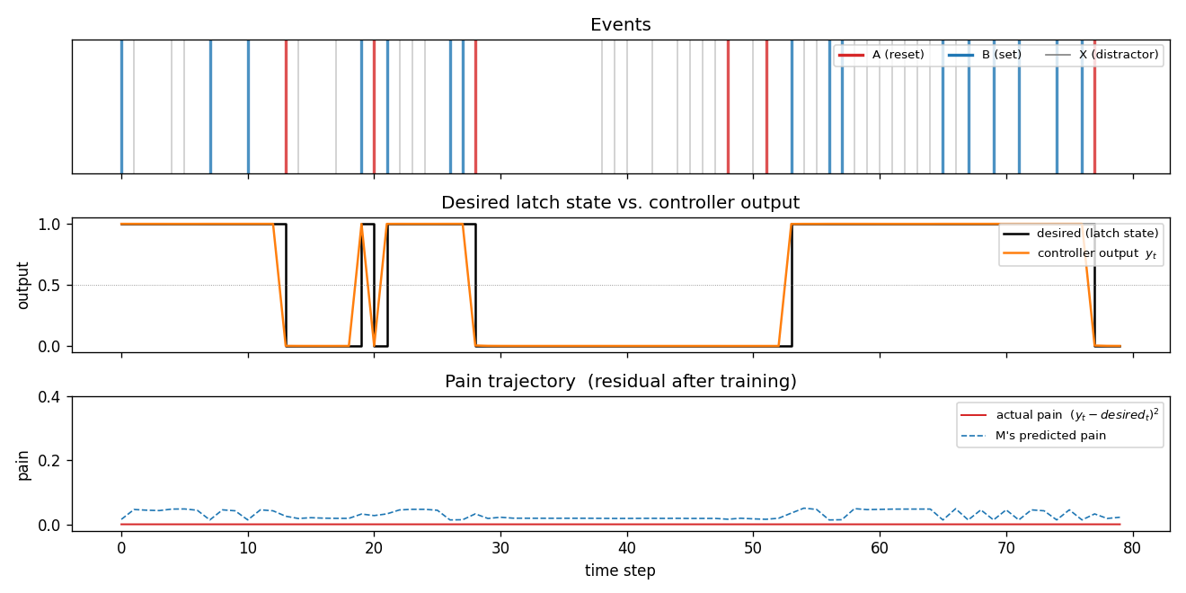
A fresh 80-step episode (different from training). The middle panel shows the
desired latch state (black step) overlaid with the controller’s continuous
output y_t (orange). After every A the controller drives y_t to 0
within one step; after every B it drives y_t to 1 and holds through
arbitrary stretches of X distractors until the next A. The bottom panel
shows actual pain (red) and M’s predicted pain (dashed blue) – both are
near zero, and they agree.
Controller weights
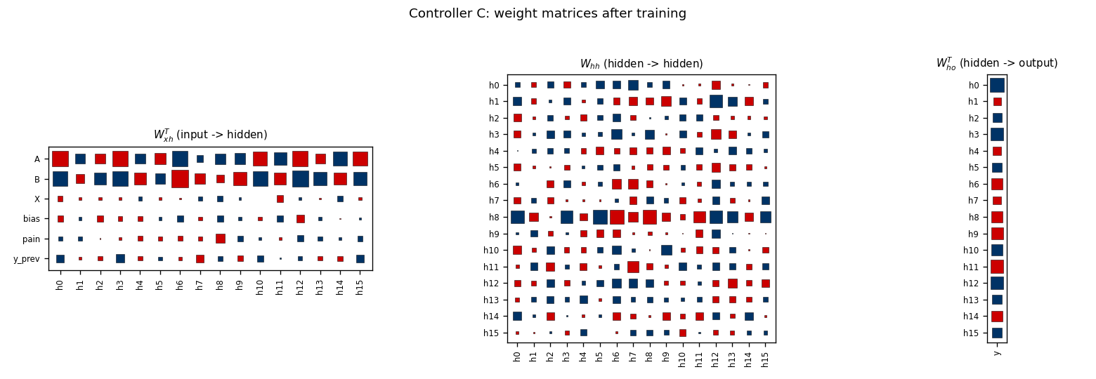
Hinton diagrams of W_xh, W_hh, W_ho after 3000 outer steps. The input
weight matrix shows large coefficients on the A and B channels (the
events that change latch state) and a strong column on y_prev – the
controller has learned that its own previous output is the cleanest cue for
maintaining the current latch state across distractors. The bias and pain
channels carry less weight once the latch behaviour is internalised in
hidden state.
World-model weights
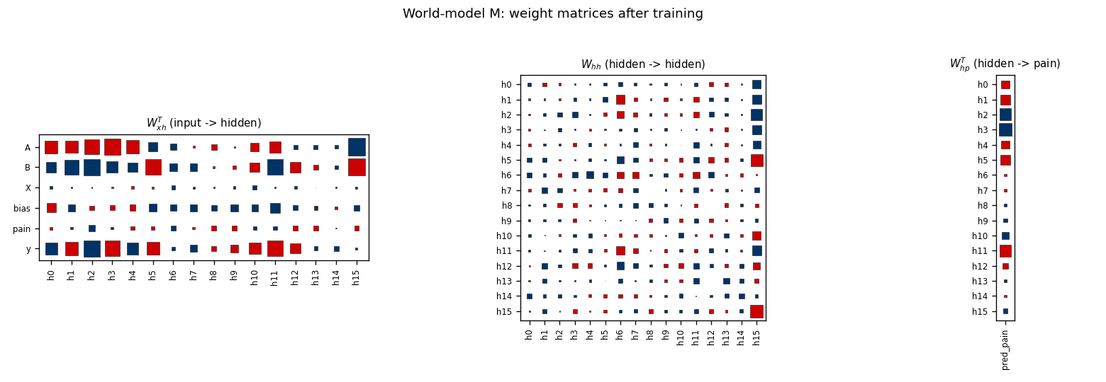
M’s W_xh puts substantial weight on y (the action channel; rightmost
row of the input panel) – this is the channel through which C’s gradient
will flow when we back-prop predicted pain into C. M’s recurrence W_hh
is dense and is the bit that lets M track the latch state from event
history.
Pain landscape
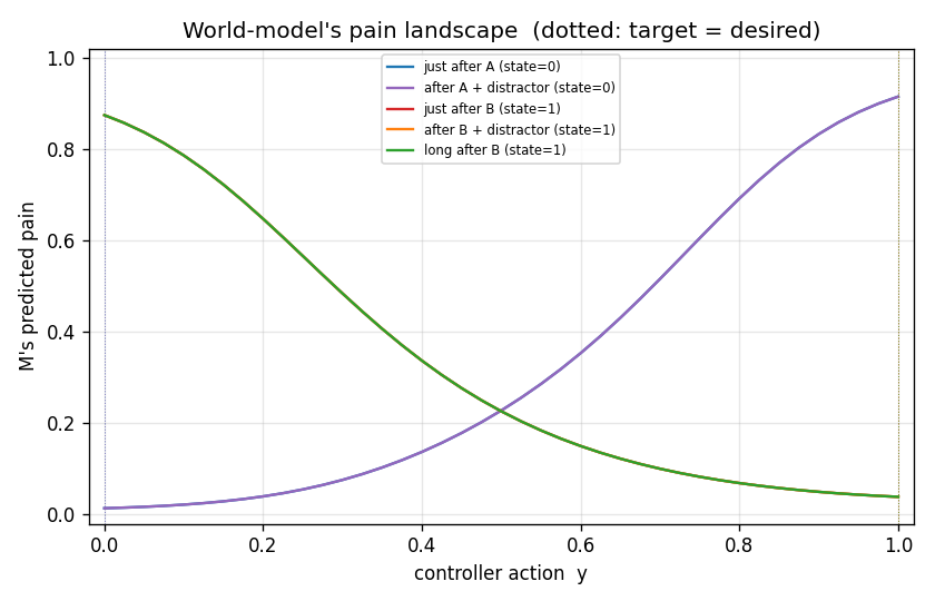
M’s predicted pain as a function of action y for five canonical latch
contexts (just after A, after A+distractors, just after B, after
B+distractors, long after B). The colored vertical dotted lines mark the true
desired output for each context. M has learned a clean upward-facing bowl
in y whose minimum sits at the correct latch target – which is exactly
what makes the gradient d pred_pain / d y a usable training signal for C.
Deviations from the original
- BPTT instead of RTRL. FKI-126-90 / IJCNN 1990 used real-time recurrent
learning (online unrolled gradient). This stub uses fixed-length BPTT over
episodes of
T=20. For independent fixed-length episodes the two are mathematically equivalent; BPTT is much simpler to implement and roughlyT xcheaper per gradient. - Truncated M-side BPTT for the C update. When backpropagating
sum_t pred_pain_tthroughMintoC, we use only the local jacobiand pred_pain_t / d y_tand zero out the recurrent gradient throughM’s hidden state. The paper’s section 6 (“Type A heuristic”) describes this shortcut. Full BPTT throughMaccumulates noise fromM’s imperfect long-horizon predictions and destabilisesCin our hands. - Random-policy rollouts for M’s training data. Each outer step we
generate one uniform-random action rollout and use it as
M’s training batch (the C-rollout is only used forC’s update, not for trainingM). Without this,Monly ever sees actions fromC’s current policy – typically a saturating sigmoid output near 0 or 1 – andM’s gradientd pred_pain / d ybecomes ill-calibrated for off-policy actions, which is exactly the regimeC’s update needs. The 1990 paper trainedMandCon the same on-policy stream and apparently lived with the resulting instability (6/10 solve rate). - Adam, not vanilla SGD. Step size
1e-2forM,5e-3forC. Per- parameter rescaling is a 2014 invention and not in the original paper, but has no bearing on the algorithmic claim (“BP through differentiable world model into a controller”). - Gradient norm clipped at 1.0 on each update.
- Smaller scale. Hidden size 16 for both nets, episode length 20, 3000
outer steps. The 1990 paper budgeted 10^6 steps. Same algorithm, much
smaller compute – the current state of
M’s pain landscape andC’s weight matrices both look qualitatively as the paper describes. - Fully numpy, no
torch. Per the v1 dependency posture.
Open questions / next experiments
- The original FKI-126-90 technical report is not retrievable in original form online; descriptions here are reconstructed from the 1990 IJCNN paper, the 1991 Curious model-building control systems IJCNN paper, and the 2020 Deep Learning: Our Miraculous Year 1990-1991 retrospective. The exact per-step training curve in Schmidhuber 1990 may differ from this stub’s curves; the 6/10 vs 10/10 success-rate gap should be cross-checked against the original report once it surfaces.
- The Type A truncation makes the stub converge but loses the credit-
assignment story across long lags. With full BPTT through
M, can we recover stability via betterMcalibration (more random-policy rollouts, higher-capacityM, ensembling)? This is the right experiment for v2. - Replacing
Cwith an LSTM (the 1997 successor on this exact problem family) is a clean follow-up. The flip-flop is the canonical task LSTM was built for; the gap between vanilla-RNN+BP-through-world-model (this stub) and LSTM with the same world-model loop is a useful diagnostic for v2’s data-movement comparison. - The flip-flop’s
desired_tis a function the world-modelMis implicitly forced to learn. WithT=20it’s easy; pushingTto hundreds with arbitrary inter-event lags would test whetherM(and through it,C) can still latch. Vanilla-RNNMis expected to break first – another natural v2 experiment, and the place where the 1991 vanishing-gradient story shows up. - In v2, instrument both networks under ByteDMD to compare the data-movement cost of the two-network world-model loop against single-network direct BP. The flip-flop is small enough that the absolute numbers will fit in L1-cache budget, which makes the ratio the meaningful quantity.