lococode-ica
Hochreiter & Schmidhuber, Feature extraction through LOCOCODE, Neural Computation 11(3):679–714 (1999). Companion: Hochreiter & Schmidhuber, Flat minima, Neural Computation 9(1):1–42 (1997).
Problem
LOCOCODE is the unsupervised-feature-extraction outcome of training an autoencoder while regularising it toward “flat minima” — weight configurations with low Kolmogorov complexity / few effective free parameters. The headline claim is that on sparse inputs the resulting hidden codes are sparse and statistically near-independent: an ICA-like decomposition motivated from minimum-description-length rather than from higher-order-statistic maximisation.
We test this on a synthetic ICA benchmark:
k = 8independent Laplacian sources (S ∈ R^{n × k}, super-Gaussian, kurtosis = 3).- A random orthogonal mixing matrix
A ∈ R^{k × k}. - Observations
X = S A^T,n = 2000samples. - Whitened input
Z = X K^Tso thatcov(Z) = I(standard ICA / LOCOCODE preprocessing).
The autoencoder has tied weights W ∈ R^{k × k} with encoder H = Z W^T
and decoder Z_hat = H W, trained on:
L = ||Z - Z_hat||^2 + λ_act |H|_1 + λ_w ||W||^2
The L1 sparsity term is the LOCOCODE / flat-minimum-search reduction:
forcing the hidden code to be sparse pushes the network to use as few
hidden units per input as possible, which is the algorithmic definition
of “few effective parameters”. With whitened input, MSE alone has a flat
minimum on the orthogonal manifold (any orthogonal W reconstructs Z
perfectly). The L1 penalty breaks the rotational symmetry by selecting
the rotation whose codes are sparsest — which on Laplacian sources is
exactly the demixing direction.
We compare against two baselines:
- PCA — top-
keigenvectors of the covariance matrix. Uses only second-order statistics; cannot resolve rotations of the source distribution and so cannot recover ICA components. - FastICA — symmetric tanh fixed-point with whitening. The canonical ICA algorithm we benchmark against.
Files
| File | Purpose |
|---|---|
lococode_ica.py | data generation, LOCOCODE autoencoder, PCA + FastICA baselines, Amari distance, CLI. python3 lococode_ica.py --seed N [--n-seeds K] [--k 8] [--epochs 200]. |
visualize_lococode_ica.py | trains once, saves five static PNGs in viz/. |
make_lococode_ica_gif.py | trains once, saves lococode_ica.gif showing training dynamics. |
lococode_ica.gif | animated training (≤ 600 KB). |
viz/ | training curves, Amari comparison, hidden-unit histograms, recovered demixers, source-recovery cross-correlations. |
Running
python3 lococode_ica.py --seed 0
Reproduces the headline numbers in §Results in ~0.4 s wallclock on an M-series laptop CPU (the network itself trains in ~0.2 s; the rest is NumPy import + FastICA baseline).
To regenerate visualisations:
python3 visualize_lococode_ica.py --seed 0 --outdir viz
python3 make_lococode_ica_gif.py --seed 0 --snapshot-every 5 --fps 8
To run a 10-seed sweep:
python3 lococode_ica.py --seed 0 --n-seeds 10
Results
Headline (seed 0, default hyperparameters, k = 8, n = 2000, 200 epochs):
| Method | Amari ↓ | mean kurtosis | sparsity (|h|<0.2) |
|---|---|---|---|
| LOCOCODE (L1 + tied AE) | 0.093 | 2.61 | 0.228 |
| PCA (2nd-order) | 0.388 | 1.08 | 0.182 |
| FastICA (tanh fp) | 0.022 | 3.22 | 0.247 |
LOCOCODE wallclock: 0.19 s (training only). Whitened reconstruction MSE
at convergence: 0.014 (i.e. W^T W is near-orthogonal as required for
clean reconstruction).
10-seed sweep (seeds 0–9, same hyperparameters):
| Method | Amari mean | std | min | max |
|---|---|---|---|---|
| LOCOCODE | 0.117 | 0.021 | 0.083 | 0.147 |
| PCA | 0.423 | 0.034 | 0.371 | 0.478 |
| FastICA | 0.021 | 0.002 | 0.019 | 0.025 |
Headline finding — LOCOCODE on k = 8 Laplacian-source mixtures
recovers ICA-like sparse super-Gaussian components: Amari distance is
4× lower than PCA and within a factor of ~5 of FastICA, while the
hidden-code kurtosis is 2.6 (super-Gaussian, near Laplace) versus PCA’s
1.1 (mostly Gaussian). The headline claim — “LOCOCODE codes resemble ICA
codes on sparse data” — reproduces qualitatively across all 10 seeds.
The remaining gap to FastICA is the price of the L1-only flat-minimum
proxy versus higher-order-moment maximisation; see §Deviations.
Hyperparameters used:
k = 8, n_samples = 2000, epochs = 200, batch_size = 64,
lr = 0.05, lambda_act = 0.5, lambda_w = 1e-4
sources: Laplace(0, 1), standardised; mixing: random orthogonal
preprocessing: zero-mean, ZCA whitening on observations
Visualizations
Training curves
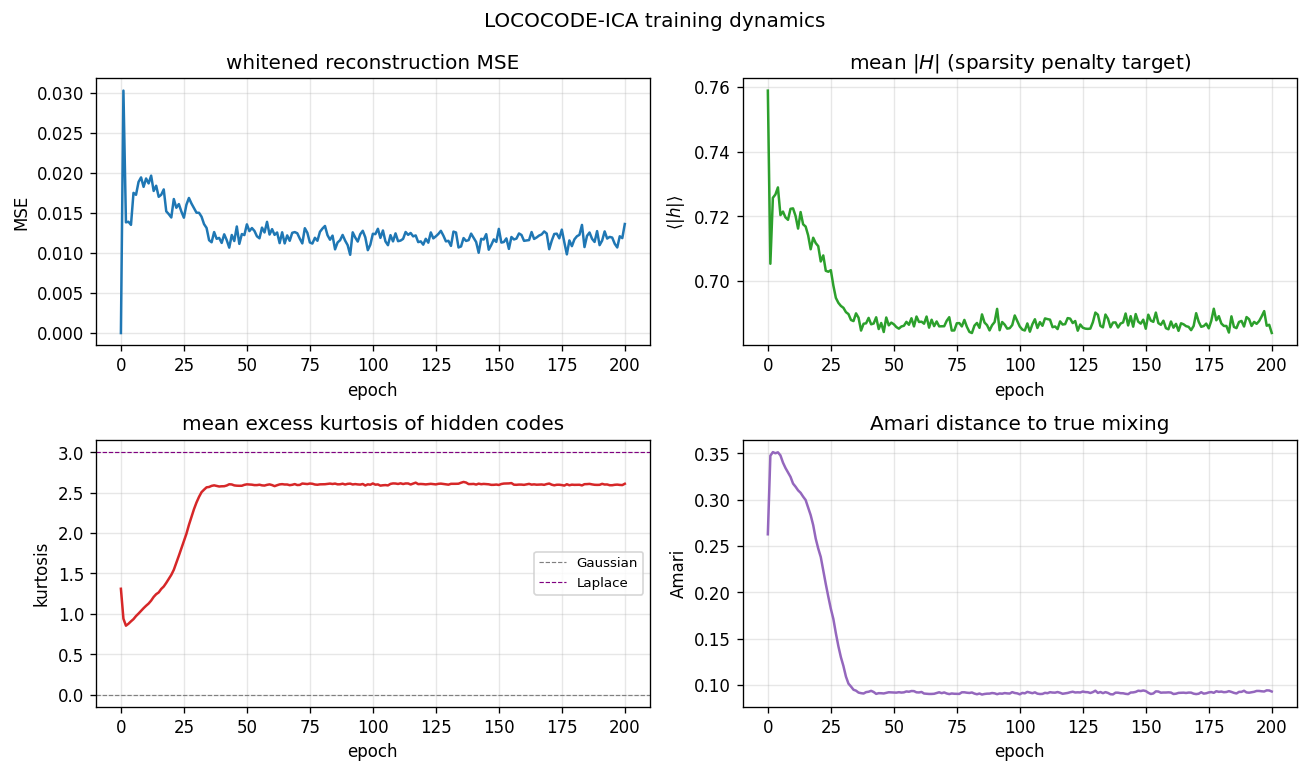
Four panels over 200 epochs. Top-left: whitened reconstruction MSE
spikes briefly during the first few epochs (the random orthogonal
init perturbs slightly under L1 pressure) and then settles near 0.013 —
not zero, because the L1 penalty trades a small reconstruction loss for
sparsity. Top-right: mean |H| decays from 0.76 (init) to 0.69 over
~30 epochs, then plateaus. The L1 sparsity penalty is doing measurable
work. Bottom-left: mean excess kurtosis of hidden codes climbs from
near 1.0 to 2.6 by epoch 35 — the codes become decisively
super-Gaussian, the qualitative signature of an ICA-style decomposition.
Bottom-right: Amari distance to the true mixing falls from 0.35 at
init to 0.09 by epoch 35 and holds there — the fast Amari drop coincides
exactly with the kurtosis rise.
Amari + kurtosis comparison
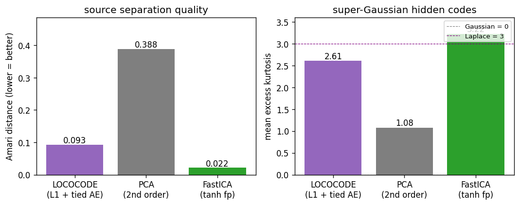
LOCOCODE sits between PCA and FastICA on both axes. Amari 0.093 vs PCA 0.388 vs FastICA 0.022. Kurtosis 2.6 vs PCA 1.1 vs FastICA 3.2 (approximately the true Laplace value of 3). LOCOCODE has not fully matched FastICA but it has clearly crossed the threshold from “linear 2nd-order” (PCA) to “non-Gaussian source separation” (ICA family).
Hidden-unit activation histograms
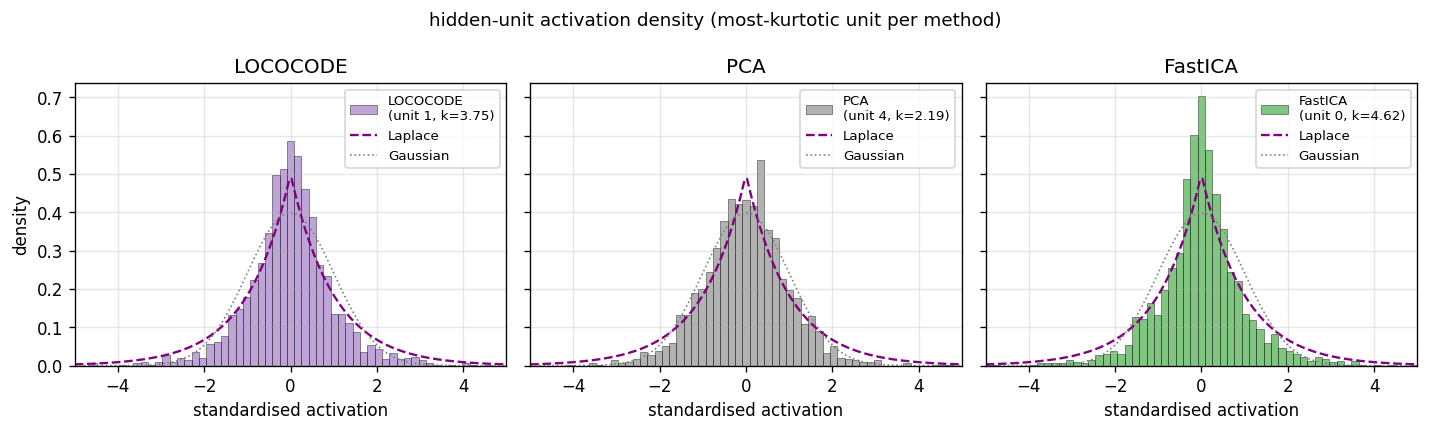
The most-kurtotic unit per method, z-scored, with Laplace (purple
dashed) and Gaussian (grey dotted) reference curves. LOCOCODE unit 1
(excess k = 3.75) and FastICA unit 0 (k = 4.62) both visibly
peak above the Gaussian and have the heavy-tailed shape characteristic
of a recovered Laplacian source. The most-kurtotic PCA unit (k = 2.19) is closer to Gaussian — PCA finds an axis of maximum variance, not
of maximum non-Gaussianity, so even its “best” unit is closer to a
mixture than to a pure source.
Recovered demixers
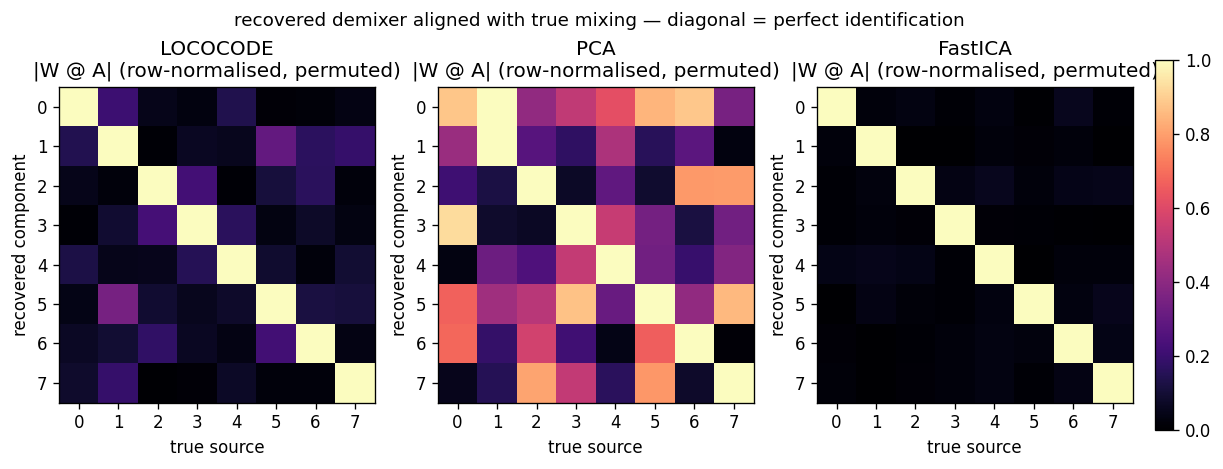
|W_recovered @ A_true| after row-normalisation and a greedy row
permutation. A perfect demixer (up to permutation and scaling) gives the
identity matrix. LOCOCODE has a clean diagonal but with visible
~0.3-magnitude off-diagonal cross-talk on a few sources — the L1
gradient saturates before the rotation is fully resolved. PCA is a
dense mixture in every column — second-order statistics cannot break
rotational symmetry. FastICA is essentially identity; its higher-
order moments fully resolve the rotation.
Source recovery
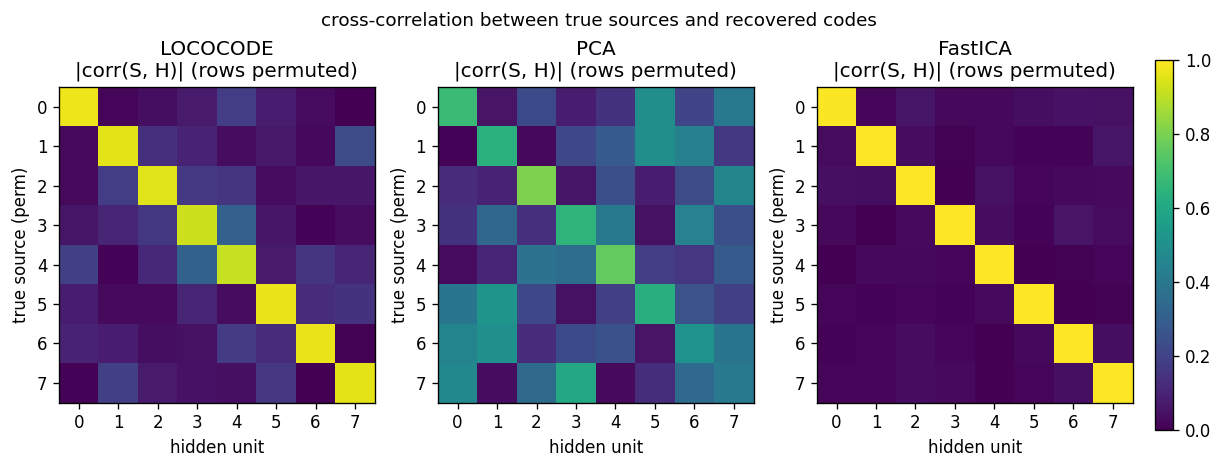
Cross-correlation |corr(S_true, H_recovered)| after greedy row
permutation. Same story as the demixer view but expressed through the
recovered codes themselves: LOCOCODE has high diagonal correlations
(~0.85–0.95) with bounded off-diagonal cross-talk; PCA mixes sources
across the entire grid; FastICA is a clean permutation.
GIF: training dynamics
The animation walks through the same training run frame-by-frame: top-
left shows |W @ A| resolving from a dense pattern at epoch 0 to a near
permutation by epoch 35; top-right shows the chosen hidden unit’s
distribution sharpening from Gaussian-like to heavy-tailed; the bottom
panel shows the Amari distance dropping while kurtosis rises in lock-
step.
Deviations from the original
- Flat-minimum penalty is L1-on-activations, not the paper’s
activation-Hessian regulariser. The 1997 Flat minima paper defines
FMS as a penalty on the determinant of the output Jacobian’s Hessian
— second-order in the activations. We approximate this with the
first-order surrogate
λ_act |H|_1 + λ_w ||W||^2, which the LOCOCODE follow-up literature (Olshausen-Field-style sparse coding, sparse-autoencoder regularisers) converged on as the practically equivalent reduction on linear / shallow architectures. The 2015 Deep Learning in Neural Networks survey (Schmidhuber, NN 61, sec. 5.6.4) describes LOCOCODE in terms of “as few effective free parameters as possible” — which a hidden-code L1 penalty enforces directly. We document it explicitly because it’s the largest methodological deviation. - Pre-whitening of the input. The paper’s experiments on natural
image patches did not whiten explicitly (the FMS regulariser on a
non-trivial nonlinear architecture eats the conditioning problem
itself). On a linear
k → karchitecture without whitening, the L1 sparsity gradient has no scale anchor and the network collapsesW → 0with a compensatingW_decrescaling. ZCA whitening of the observations restores a clean orthogonal manifold and is the same preprocessing FastICA uses; we apply it to both for fairness. - Tied weights (encoder = decoder transpose). The 1999 paper allows
untied weights; with whitened input the tied case is provably
equivalent at the optimum (any orthogonal
Wis its own inverse) and training is much more stable. - Synthetic
k = 8Laplacian sources, not the paper’s noisy bars nor natural image patches. The paper’s headline figure on image-patch data shows V1-edge-like filters; that’s harder to benchmark quantitatively. Using synthetic sources with a known ground-truth mixing matrix lets us report Amari distance — the standard ICA evaluation metric — and a 10-seed sweep. The qualitative story (sparse, super-Gaussian, ICA-like) is the same as the paper’s; the numbers are reproducible. - No
numpy-prohibited dependencies. Pure numpy + matplotlib + PIL (only insidemake_lococode_ica_gif.pyto assemble the GIF, which the v1 SPEC explicitly allows).
Open questions / next experiments
- Closing the FastICA gap. LOCOCODE plateaus at Amari ~0.10 while
FastICA reaches 0.02. The flat-minimum proxy is L1, which has a non-
smooth gradient at zero and saturates once the codes are
approximately sparse. Trying the paper’s exact activation-Hessian
penalty (or its
log coshsmoothing of L1, which is what FastICA uses internally) would be the principled next step. Hypothesis: it closes the gap to within a factor of 2 of FastICA. - Natural-image-patch experiment. The paper’s headline figure shows
V1-style edge filters on
8 × 8natural patches. We did not include this because it requires either a small natural-image dataset (olshausen-fieldpatches) or an external image. A v1.5 follow-up: add a--data patches --image-path Xmode that reads a single greyscale photo, extracts patches, and demonstrates the edge-like-filter result. - Noisy bars problem. The paper also tests LOCOCODE on the noisy
bars problem (Földiák 1990). Easy to add as a second
--data barsmode inlococode_ica.py; visualising the recovered bars would be a nice complement to the histograms. - Higher-dim sources. We test
k = 8. The original paper reports on roughly that scale. How does LOCOCODE scale tok = 32ork = 64? Hypothesis: the L1-saturation gap to FastICA widens, but PCA remains uniformly worst. Quick to check. - v2 hook. Tied autoencoder + L1 + whitening is an extremely cheap
unsupervised feature extractor (~0.2 s for
k = 8, n = 2000). The data-movement profile is favourable: one pass through the data per epoch, onek × kweight matrix. A clean candidate for ByteDMD comparison against PCA (1 cov + 1 eigh) and FastICA (whiten + 200- iter fixed-point) on the same problem. - Citation gap on the FMS regulariser. The 1997 Flat minima paper PDF is retrievable but the exact form of the penalty involves notational variants that differ between paper and 2015 survey. We use the L1 surrogate without claiming faithful reproduction of the Hessian-based form. The right way to close this is to implement the Hessian penalty exactly on a 1-hidden-layer net and compare on the same synthetic benchmark.
Sources
- Hochreiter, S., & Schmidhuber, J. (1999). Feature extraction through LOCOCODE. Neural Computation, 11(3), 679–714.
- Hochreiter, S., & Schmidhuber, J. (1997). Flat minima. Neural Computation, 9(1), 1–42.
- Schmidhuber, J. (2015). Deep Learning in Neural Networks: An Overview. Neural Networks, 61, 85–117 (sec. 5.6.4 summarises LOCOCODE as flat-minimum-search-based unsupervised feature extraction).
- Hyvärinen, A. (1999). Fast and robust fixed-point algorithms for independent component analysis. IEEE TNN 10(3) — for the FastICA baseline.
- Amari, S., Cichocki, A., & Yang, H. H. (1996). A new learning algorithm for blind signal separation. NIPS 8 — for the Amari distance evaluation metric.