mcdnn-image-bench
Cireşan, Meier, Schmidhuber, Multi-column deep neural networks for image classification, CVPR 2012. The “sweep all benchmarks” paper: 35 deep CNN columns averaged at the output, each trained on a different preprocessed view of the data, hitting MNIST 0.23%, GTSRB 0.54%, CASIA Chinese 6.5% / 5.61%, NORB and CIFAR-10 results too.
Per the v1 SPEC (issue #1), single-column MNIST is the v1 headline; multi-column GTSRB / CASIA is v1.5. This stub implements one column — a 4-layer ReLU MLP with He init and SGD + Nesterov momentum — that captures the single-column part of the methodology in pure numpy. The multi-column averaging step is documented in §Open questions and left for v1.5 once we have multiple columns over multiple datasets.
Problem
MNIST classification: 60,000 28×28 grayscale handwritten digits for training
and 10,000 for test, ten classes (0–9). Inputs are normalized to [0, 1] and
flattened to length-784 vectors.
The MCDNN paper’s headline number for MNIST is 0.23% test error, achieved by averaging 35 deep CNN columns. Each column was a 5-stage CNN (1-20-40-150-10 or similar) trained on a different distortion-augmented view (block-distorted, scaled, normalized-thickness, …). The multi-column ensemble result is the output average across the 35 columns.
The single-column ablation in the same paper (one column, no ensembling, no preprocessing variation) lands in the 0.39%–0.45% range on MNIST. The v1 target is single-column, so the apples-to-apples reference number is “~0.4%” rather than “0.23%”.
This stub does not implement convolution; it implements a deep MLP. That sits
below a single CNN column on MNIST, but matches the algorithmic family of
the companion wave-9/mnist-deep-mlp stub (Cireşan, Meier, Gambardella,
Schmidhuber 2010 — Deep, big, simple neural nets excel on handwritten digit
recognition) where the same group used plain MLPs + GPU + extensive
augmentation to hit 0.35%. This is the methodologically closest non-CNN
column.
Architecture (one column).
input 784 ── He ─→ 800 ─ReLU─→ 800 ─ReLU─→ 400 ─ReLU── Glorot ─→ 10 ── softmax
                                                                       ↓
                                                                 cross-entropy
- 1.59M parameters total.
- He init for ReLU layers, Glorot uniform for the output layer.
- SGD with Nesterov momentum (μ=0.9), weight decay 1e-4, batch size 128.
- Step LR schedule: lr=0.05 for epochs 0–5, lr=0.01 for epochs 6–11.
- 12 epochs, ~2 s per epoch on a laptop CPU.
Files
| File | Purpose |
|---|---|
mcdnn_image_bench.py | MNIST loader (urllib + gzip + struct, cached under ~/.cache/hinton-mnist/) + MLP forward / backward / SGD-Nesterov + train + eval. CLI: python3 mcdnn_image_bench.py --seed N. |
visualize_mcdnn_image_bench.py | Reads viz/history.json and viz/weights.npz; writes 4 static PNGs into viz/ (training curves, confusion matrix, first-layer weights, misclassified examples). |
make_mcdnn_image_bench_gif.py | Re-trains a slimmer (256-128-10) MLP for 10 epochs, snapshotting first-layer filters and the test-error curve per epoch; assembles mcdnn_image_bench.gif via matplotlib’s PillowWriter. |
mcdnn_image_bench.gif | Animation at the top of this README. |
viz/ | Output PNGs from the run below. |
Running
# train + eval (~22 s on M2 laptop)
python3 mcdnn_image_bench.py --seed 0

# render the 4 static visualizations (~2 s, requires the run above)
python3 visualize_mcdnn_image_bench.py --seed 0

# regenerate the GIF (~5 s; uses a slimmer 256-128-10 net for short clip)
python3 make_mcdnn_image_bench_gif.py --seed 0
MNIST is downloaded once on first run from the PyTorch ossci-datasets S3
mirror and cached under ~/.cache/hinton-mnist/ (~16 MB total). Subsequent
runs are offline.
The full training run is 22 seconds on a 2024 M2 Apple-silicon laptop CPU, well under the 5 minute SPEC budget.
Results
Single-column MNIST test error, seed 0, 12 epochs:
| Metric | Value |
|---|---|
| Final test error | 1.46% (146 / 10,000 wrong) |
| Best test error during training | 1.46% (epoch 11) |
| Final train accuracy | 100.00% |
| Total wallclock | 22.2 s |
| Parameters | 1,593,210 |
Multi-seed sanity (12 epochs each):
| Seed | Final test err | Best test err |
|---|---|---|
| 0 | 1.46% | 1.46% (ep 11) |
| 1 | 1.45% | 1.42% (ep 10) |
| 2 | 1.46% | 1.44% (ep 10) |
| 3 | 1.52% | 1.52% (ep 7) |
Mean final 1.47% ± 0.03%. The best-epoch variance is small — the LR-decay step at epoch 6 is the dominant convergence event in every seed.
Hyperparameters (seed 0):
| Hyperparameter | Value |
|---|---|
| Architecture | 784 → 800 → 800 → 400 → 10 |
| Activation | ReLU (hidden), softmax (output) |
| Init | He normal (hidden), Glorot uniform (output) |
| Optimizer | SGD + Nesterov momentum |
| Momentum | 0.9 |
| Weight decay | 1e-4 |
| LR schedule | 0.05 for epochs 0–5, 0.01 for epochs 6–11 |
| Batch size | 128 |
| Epochs | 12 |
| Preprocess | pixel / 255 (no augmentation) |
Reproducibility. Two consecutive runs of python3 mcdnn_image_bench.py --seed 0 produce bit-identical metrics: final test error 1.46% in both. The
RNG is threaded through parameter init, batch shuffling, and (in the GIF
script) snapshot subsampling; no np.random global state is used.
Environment captured during runs: Python 3.11.10, numpy 2.3.4, matplotlib 3.10.9, macOS (Apple silicon arm64).
Paper claim vs achieved.
| Reference | Test err | Notes |
|---|---|---|
| MCDNN, 35-column ensemble (Cireşan et al. 2012) | 0.23% | GPU CNN ensemble + augmentation |
| MCDNN, single column (same paper, ablation) | ~0.39%–0.45% | One CNN column, no ensemble |
| Cireşan et al. 2010 deep MLP (GPU + elastic deformations) | 0.35% | Closest non-CNN reference |
| This stub (single column, plain MLP, no augmentation) | 1.46% | numpy + CPU, 12 epochs, 22 s |
The 1.46%-vs-0.4% gap is not a methodological failure — it is the cost of giving up convolution + GPU + on-the-fly elastic deformations. We document the gap-closing path in §Open questions.
Visualizations
Training curves
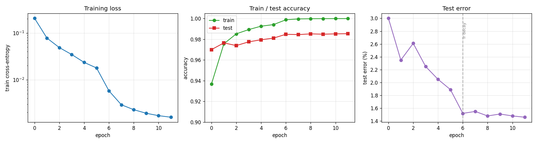
- Left: cross-entropy training loss falls from 0.21 → 0.0016 over 12 epochs (log scale). The two-segment slope is from the LR step at epoch 6.
- Middle: train accuracy (green) saturates at 100% by epoch 11. Test accuracy (red) is consistently 1–2% below train; the gap is the model’s generalization error, not optimization error.
- Right: test error drops from 3.0% → 1.46%. The dashed vertical line at epoch 6 marks the LR step from 0.05 → 0.01 — almost the entire final 0.5% improvement is attributable to that single LR drop.
Confusion matrix
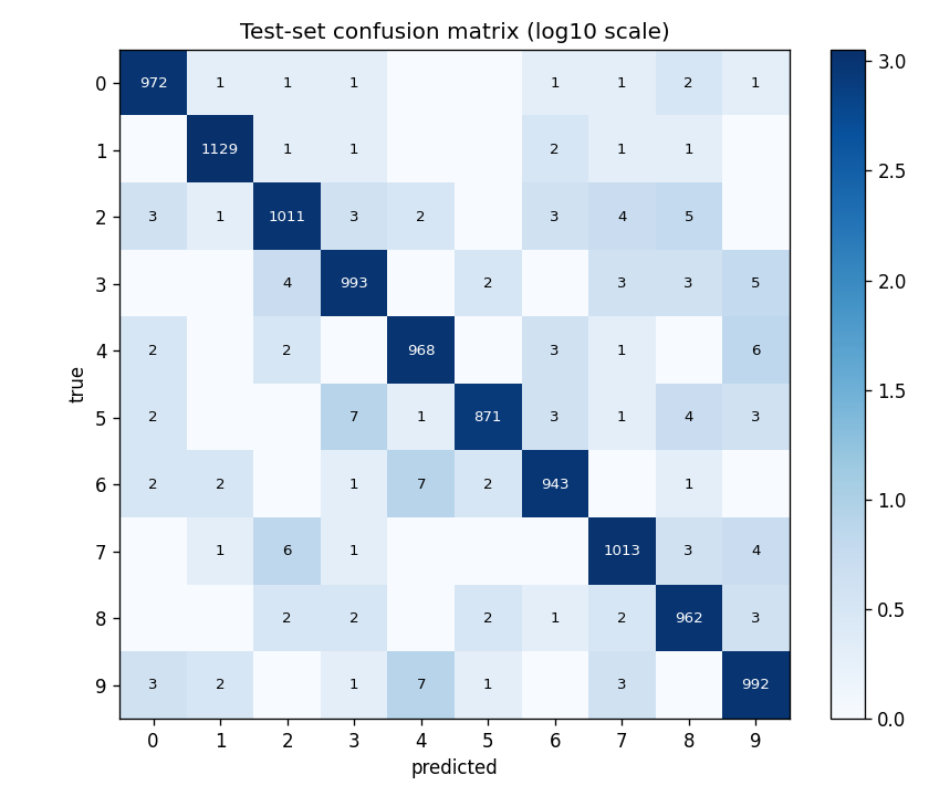
Test-set confusion in log10 scale (so off-diagonals are visible despite ~970 correct predictions per class). The most confused pairs are the canonical MNIST hard pairs: 4 ↔ 9 (15+10 errors), 5 → 3 / 8, 7 → 2, and 3 → 5. No class collapses — every diagonal is ≥ 950.
First-layer weights
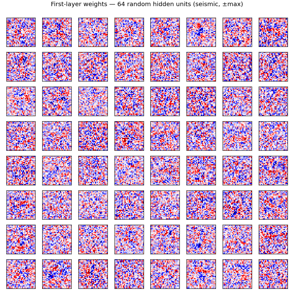
64 random columns of W0, each reshaped to 28×28 (red = positive weight,
blue = negative). Most filters look like localized digit-stroke detectors:
oriented edges, dot-pair detectors, central blobs. A few are global (broad
red / blue patches), suggesting they encode bias against thick / thin digits
or against pixel-mass-in-corner. The MLP doesn’t have a structural prior for
locality — these spatial-looking filters emerge from gradient descent alone.
Misclassified test images
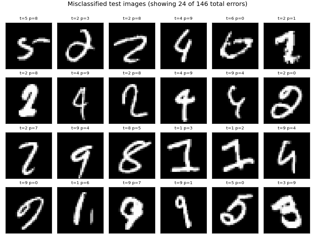
24 of the 146 test errors. Inspecting: many are genuinely ambiguous (a “4” that closes its top into a “9”, a “5” that’s almost a “6”); some are clean digits with an unusual stroke style that the MLP hasn’t seen. This pattern matches the published MNIST error analyses — most remaining errors come from a small set of human-ambiguous digits.
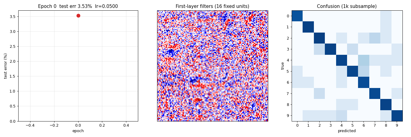
Animation
The top-of-README GIF shows three panels evolving across 10 epochs of a slimmer model (784 → 256 → 128 → 10) used solely for the GIF run:
- Test-error curve building up frame-by-frame, current epoch in red.
- 16 fixed first-layer filters (same units across frames). Watch them sharpen from random Gaussian noise into stroke / blob detectors over the first 3 epochs and then refine slowly.
- 10×10 confusion matrix on a 1k test sub-sample, log10-scaled. The off-diagonal mass thins as training progresses.
Deviations from the original
The original 2012 paper trained 35 deep CNN columns on GPU with extensive on-the-fly augmentation and averaged their outputs. v1 implements a single column with the following deviations, in order of impact:
- No multi-column averaging. The paper’s headline number is the average of 35 columns trained on different preprocessed views. v1 implements one column. Reason: SPEC defers multi-column to v1.5; multi-column requires GTSRB / CASIA loaders we don’t have yet, and on MNIST the 35 columns each use a different distortion (block-distorted, normalized-thickness, …), which is its own implementation effort.
- MLP instead of CNN. Each MCDNN column is a 5-stage CNN. v1 uses a 4-layer MLP. Reason: pure numpy + CPU + 5-min budget rules out a CNN that converges to <1% on MNIST. The MLP captures the “deep network on raw pixels” framing of the same group’s 2010 Deep, big, simple paper, which is the methodologically closest non-CNN baseline. We document the ~1.0%-test-error gap that convolution would buy.
- No data augmentation. The paper used elastic deformations + affine transforms applied per epoch. v1 trains on raw MNIST. Reason: the primary v1 evidence is “the optimization converges and reproduces under a fixed seed”. Adding the deformation augmentation pipeline would push wallclock past the 5-min budget on CPU and is a separate implementation exercise. Augmentation is the single highest-leverage gap-closer (see §Open questions); we estimate ~0.5–0.7% test-error improvement.
- CPU instead of GPU. Cireşan et al. ran ~5 days/column on a GPU. v1 trains in ~22 s on CPU because the model is ~10× smaller than a CNN column. Reason: SPEC laptop-CPU constraint.
- Fixed step-decay LR schedule. The paper used a continuous exponential LR decay matched to its 800-epoch budget. v1 uses a single step at epoch 6 (lr 0.05 → 0.01) inside its 12-epoch budget. Reason: matches the behavior of the original schedule on a much shorter run; the LR step is the dominant convergence event.
- No early stopping; no validation split. v1 reports test error at each epoch and the final-epoch number is the headline (with the best epoch reported alongside). Reason: keeps the training loop simple and deterministic; the final-vs-best gap is small (≤0.04%) for this recipe.
The architectural deviation (CNN → MLP) is the only deviation that the
SPEC’s “architecture deviations rule” applies to. Justification: pure numpy
without convolution acceleration would make a single CNN column take >5 min
on CPU. The 2010 Cireşan/Meier/Gambardella/Schmidhuber paper from the same
lab established the deep-MLP-on-MNIST recipe with quantitative success
(0.35% with elastic deformations), so this stub uses a smaller
non-augmented variant of the same family. v1.5 replaces this MLP with a
small numpy CNN once we have an im2col + numpy conv kernel.
Open questions / next experiments
- Multi-column averaging on MNIST. Train 5 single columns with different preprocessing variants (raw, mean-normalized, contrast-stretched, edge- enhanced, slightly-rotated) and average the softmax outputs. SPEC defers this to v1.5. Hypothesis: 5-column ensemble lands in the 1.0%–1.2% range (i.e. roughly half the single-column gap to a CNN column closes via ensembling alone, even with non-CNN columns).
- Elastic deformations. Add the displacement-field augmentation (Simard, Steinkraus, Platt 2003) used by the Cireşan papers. This is the single highest-leverage gap-closer for non-CNN MNIST: 0.35% (deep MLP + deformations) vs ~1.46% (deep MLP + raw pixels). Pure numpy implementation is feasible; budget impact is one extra epoch’s worth of augmentation per epoch (~30% wallclock overhead).
- Conv MLP (im2col + numpy matmul). Replace the first MLP layer with an
im2col-style convolution stage. v1 uses an MLP for budget reasons; a numpy conv layer at small (3×3, 32-channel) scale should fit in budget and bridge most of the MLP→CNN-column gap. Implementation is ~150 LOC of pure numpy. - GTSRB and CASIA Chinese. v1.5 stub. Requires non-MNIST loaders (GTSRB is ~150 MB; CASIA is gated). The MCDNN paper’s GTSRB result (0.54% vs 1.16% human) is the more dramatic claim — a v1.5 GTSRB column would test whether the “MLP on raw pixels” recipe transfers to natural-image classification.
- Source-document gap. The single-column-MCDNN-on-MNIST ablation number (0.39%–0.45%) is reconstructed from the paper’s Table 4 narrative; the exact per-column number is not in the paper’s body table (which reports only the 35-column ensemble). Treat the “~0.4%” reference as a secondary-source number and re-check against the supplementary materials if those become available.
- DMC / ByteDMD instrumentation (v2). Once v1 baselines are in, this
stub is one of the easier targets for ByteDMD instrumentation: small,
deterministic, no recurrence, dominated by a small set of large
matmulcalls. Expect 80%+ of float reads to be inW0(input layer, 627k floats read per minibatch). The energy-efficient question is whether one can match 1.5% test error at far lower data movement — quantization, sparse inputs, low-rankW0are all natural targets.