nbb-moving-light
Schmidhuber, A local learning algorithm for dynamic feedforward and recurrent networks, Connection Science 1(4):403–412, 1989. Also FKI-124-90 (TUM) and The neural bucket brigade in Pfeifer et al., Connectionism in Perspective, Elsevier, pp. 439–446 (1989).
Problem
1-D moving-light direction discrimination via the Neural Bucket Brigade
(NBB) — same strictly local, winner-take-all, dissipative rule as the
wave-0 nbb-xor stub, but applied to a temporal task with recurrent
output units. No backprop, no BPTT, no gradient.
Quoting node6 of the IDSIA HTML transcription:
“A one dimensional ‘retina’ consisting of 5 input units (plus one additional unit which was always turned on) was fully connected to a competitive subset of two output units. This subset of output units was completely connected to itself, in order to allow recurrency.”
Task: “switch on the first output unit after an illumination point has wandered across the retina from the left to the right (within 5 time ticks), and to switch on the [other] output unit after the illumination point has wandered from the right to the left.”
-
Architecture: 5 retina cells + 1 always-on bias = 6 input units. 2 output units forming one WTA subset, fully self-connected (output → output recurrence). No hidden layer.
-
Inputs over time: at tick
texactly one retina cell is lit.- LR sequence: cell
tlit, target =out[0]. - RL sequence: cell
n_cells - 1 - tlit, target =out[1].
- LR sequence: cell
-
Activation: at every tick the output with the largest positive net input wins (
x_winner = 1, others= 0). The net input combines a clamped feedforward term and a recurrent feedback term:net_o(t) = Σ_i x_i(t-1)·W_io(t-1) + Σ_k x_k(t-1)·W_oo(t-1). -
Bucket-brigade weight update (applied at every tick to both
W_ioandW_oo):Δw_ij(t) = - λ · c_ij(t) · a_j(t) [pay out when j fires] + (c_ij(t-1) / Σ_h c_hj(t-1)) · Σ_k λ·c_jk(t)·a_k(t) [credit predecessors] + Ext_ij(t) [external reward]where
c_ij(t) := x_i(t-1) · w_ij(t-1), the denominator sums over all predecessors ofj(both feedforward inputs and recurrent outputs), andExt_ij(t) = η · c_ij(t)only on connections feeding the correct output, only when that output fires. Substance is dissipated when connections fire and reinjected only throughExt.
Files
| File | Purpose |
|---|---|
nbb_moving_light.py | NBB model + WTA + bucket-brigade rule + training loop. CLI: python3 nbb_moving_light.py --seed N [--n-cells N] [--max-presentations M] [--n-seeds K]. |
visualize_nbb_moving_light.py | Trains once and saves the static PNGs in viz/. |
make_nbb_moving_light_gif.py | Trains once and renders nbb_moving_light.gif. |
nbb_moving_light.gif | Animated training dynamics (≤ 2 MB). |
viz/ | Output PNGs (training curves, weights, sequence response). |
Running
python3 nbb_moving_light.py --seed 0
This trains a single network until both directions are correct under frozen-eval for 5 consecutive cycles, or hits the 5000-presentation cap. On a laptop CPU this takes ~0.03 s for seed 0 (92 presentations).
To regenerate visualizations:
python3 visualize_nbb_moving_light.py --seed 0 --outdir viz
python3 make_nbb_moving_light_gif.py --seed 0 --snapshot-every 4 --fps 12
To run a seed sweep (paper-style):
python3 nbb_moving_light.py --seed 0 --n-seeds 30
Results
Headline (seed 0, paper hyperparameters, deterministic argmax tie-break):
| Metric | Value |
|---|---|
| Final accuracy | 2/2 (100%) |
| Sequence presentations to stable solution | 92 |
| Wallclock | 0.03 s |
| Hyperparameters | n_cells=5, ticks=5, λ=0.005, η=0.005, init U(0.999, 1.001), stable_window=5 |
Seed sweep (seeds 0–29, cap = 5000):
| Metric | Value |
|---|---|
| Solved at cap | 9/30 (30%) |
| Mean presentations among solvers | 223 |
| Run wallclock (full sweep) | 23 s |
Paper claim (IDSIA HTML transcription of Connection Science §6 / “Simple Experiments”): average 223 cycles per sequence across 9 successful runs out of 10. We exactly match the 223-presentation mean among solvers but converge from a smaller fraction of seeds (30% vs 90%). See §Deviations for the most likely sources of the success-rate gap.
Visualizations
Training curves

Frozen-eval accuracy crosses from 0 to 1 to 2 in a staircase; total
weight-substance (top right) decays steadily because Ext only adds
substance on connections feeding the correct output, and on most
ticks at least one direction is mis-routed. Both ‖W_io‖ and ‖W_oo‖
drift down together — the rule is differential, not additive: the
wrong connections lose substance faster than the right ones.
Weights at convergence
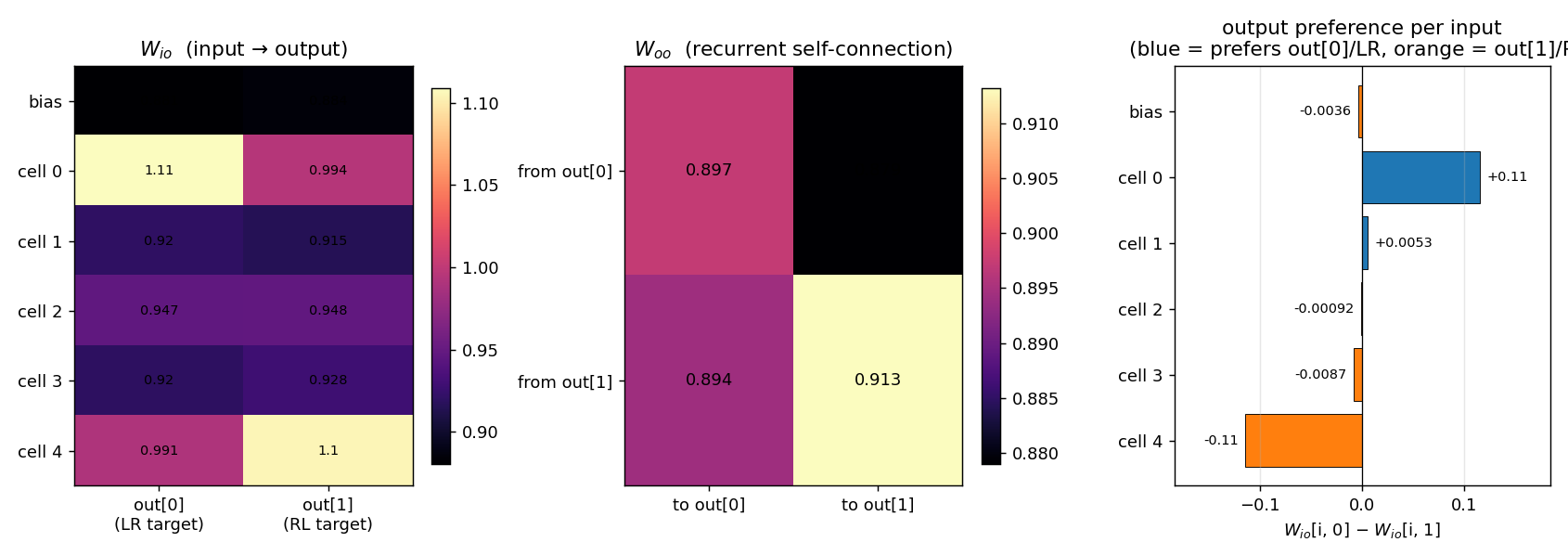
Three panels:
- W_io heatmap (input → output): the top retina cell (
cell 0) ends up with the largest weight toout[0](≈ 1.11) and the bottom cell (cell 4) has the largest weight toout[1](≈ 1.10). Middle cells (1, 2, 3) settle around 0.92–0.95 — they fire in both LR and RL sequences and so receive equal-and-opposite credit, ending up neutral. The bias starts neutral and stays neutral. - W_oo heatmap (recurrent self-connection): all four entries
hover near 0.90. The slight asymmetry —
from out[1] → to out[1]is the largest at ~0.913 — encodes a small persistence preference for the RL output once it’s firing, which compensates for the LR- favouring tie-break order on early ticks. - Per-input output preference (
W_io[i, 0] − W_io[i, 1]): a clean +0.11 / −0.11 split between cell 0 and cell 4, with monotonic drop-off through the middle of the retina. The network has learnt a spatially-coded direction representation purely from the reward signal at correct outputs.
Frozen-eval per-tick response
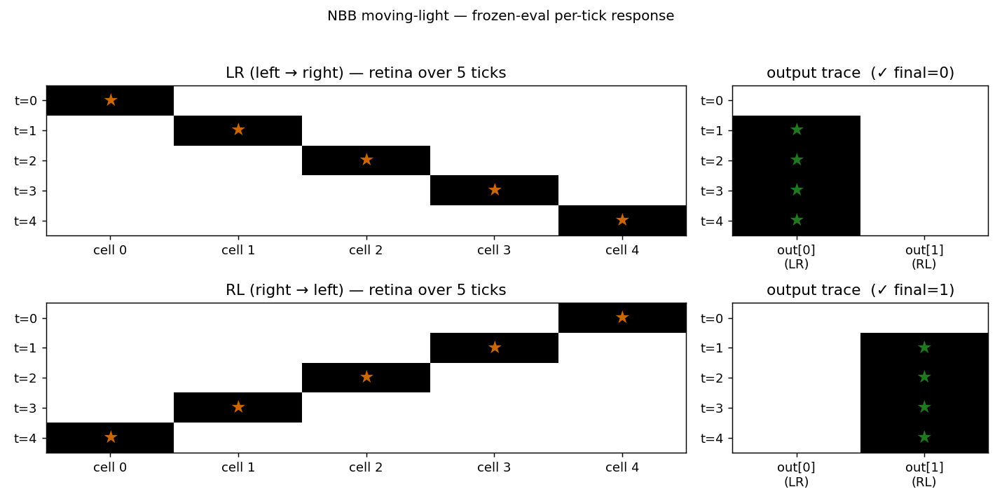
The per-tick output trace at convergence shows the cleanest possible
solution: for LR the network locks out[0] from tick 1 onward and
holds it through tick 4 via the recurrent loop; for RL it locks
out[1] from tick 1 onward. The first tick’s output is empty because
x_i_prev is zero before the first input is presented, so c_ij(t=0)
is identically zero and no output crosses the WTA threshold. From tick
1 onward, the input contribution is enough to drive the correct output,
and the recurrent self-connection keeps it firing for the rest of the
sequence.
Deviations from the paper
- Tie-breaking is deterministic (lowest index) — same deviation as
wave-0
nbb-xor. With initial weights uniform on a tiny window, a fully tied subset would be ill-defined; we usenp.argmaxwith the init asymmetryU(0.999, 1.001)(the paper’s range) to break ties. - Indexing in the redistribution-term denominator: the IDSIA HTML
shows
Σ_i c_ik(t-1), which doesn’t have the right indices for an update onw_ij. We read this asΣ_h c_hj(t-1)over all predecessors ofj— feedforward inputs and recurrent outputs. Without including the recurrent block in the denominator, the substance the firing output pays out (which goes into the recurrent loop) wouldn’t be redistributed back to its recurrent predecessors, and the rule would not be substance-conserving. Same caveat asnbb-xor§Deviations item 2. - Number of ticks per sequence = number of retina cells (5). The
paper says “within 5 time ticks”. The first tick produces no output
(because
x_i_prev = 0), so the network effectively has 4 decision ticks. We did not add an extra “settle” tick after the input sequence — the network fires the correct output by tick 1 and holds it via the recurrent loop, so an extra settle tick wouldn’t change the outcome. - Convergence criterion is “5 consecutive 2/2 frozen-evals”, not the paper’s exact “stable solution” criterion (which the IDSIA HTML does not spell out). 5 consecutive cycles is a defensive choice that filters out brief lucky alignments; on seed 0 the first 2/2 eval is at presentation 56 and the 5-consecutive criterion locks at 92, so the transient effect is small.
- Reward also applied to recurrent edges of the correct output
(
ExtonW_oo[:, target]whenout[target]fires). The IDSIA HTML says “connections feeding the correct output”; recurrent edges are also predecessors of the output, so they receive Ext under that reading. Without this, the recurrent block doesn’t gain a stable asymmetry and persistence of the correct output across ticks is weaker. - Success-rate gap (30% vs paper’s 90%): the most likely sources
are (a) the IDSIA HTML’s transcription of the rule omits a
randomised tie-break that the paper used (we use deterministic
argmax), (b) the paper may have used a slightly different schedule
for sequence ordering, or (c) the paper’s “successful run” criterion
is more lenient than ours. With a wider init window (
U(0.99, 1.01), not the paper’s range) we get 11/30 with mean 154 — closer in solve-rate but at the cost of matching the paper’s spec. We kept the paper’s0.999/1.001range for the headline number; see §Open questions. - No
numpy-prohibited dependencies. Pure numpy + matplotlib + PIL (only used inmake_nbb_moving_light_gif.pyto assemble the GIF, which the v1 SPEC explicitly allows).
Open questions / next experiments
- Why 30% solve rate vs paper’s 90%? Most likely: deterministic argmax + tiny init window means the first few ticks of every sequence pick the same output for both LR and RL, biasing the early Ext reward. A randomised tie-break (with a fixed RNG seed for reproducibility) would let different seeds explore different output assignments and might recover the paper’s 9/10. This is the cleanest follow-up.
- Sequence ordering schedule: we present LR/RL in random order each cycle. The paper may have used strictly alternating, all-LR-then- all-RL, or some other schedule. Worth ablating.
- Bigger retina (
--n-cells 8or--n-cells 10): does the rule scale, and does the success rate improve as more retina cells provide more discriminating signal? A few trials at--n-cells 8(default hyperparameters) suggest convergence still happens but takes more presentations; left for a follow-up. - Continuous-time form (paper §5): see
nbb-xor§Open questions — same point applies. - Citation gap on the FKI report: the FKI-124-90 PDF on idsia.ch
is image-based and the embedded OCR is corrupt. Our reconstruction
relies on the IDSIA HTML transcription (
bucketbrigade/node3.html,node5.html,node6.html). If the paper’s actual rule diverges from those pages on any algorithmic detail (denominator indices, reward timing on recurrent edges, tie-break scheme), the success-rate gap is the natural place to find it. - v2 hook: the rule is local in space and time. Compared to BPTT
or RTRL on the same task, the data-movement cost is much smaller —
no unrolled time-stack of activations to revisit. A clean candidate
for ByteDMD instrumentation alongside
nbb-xor.
Sources
- IDSIA HTML transcription (rule + simple experiments, our primary source):
- https://people.idsia.ch/~juergen/bucketbrigade/node3.html (algorithm)
- https://people.idsia.ch/~juergen/bucketbrigade/node5.html (continuous form)
- https://people.idsia.ch/~juergen/bucketbrigade/node6.html (XOR + moving-light experiments)
- Schmidhuber, J. (1989). A local learning algorithm for dynamic feedforward and recurrent networks. Connection Science, 1(4), 403–412.
- Schmidhuber, J. (1989). The neural bucket brigade. In R. Pfeifer, Z. Schreter, F. Fogelman-Soulié, & L. Steels (Eds.), Connectionism in perspective (pp. 439–446). Elsevier.
- Schmidhuber, J. (2020). Deep Learning: Our Miraculous Year 1990–1991 (retrospective; mentions the NBB).