pomdp-flag-maze
Schmidhuber, Reinforcement learning in Markovian and non-Markovian environments, NIPS-3 (1991), pp. 500-506. Background and corroboration in Schmidhuber 2015, Deep Learning in Neural Networks: An Overview §6.10 (POMDP RL with recurrent world models), and the Miraculous Year 1990-1991 review (2020).
Problem
A 2-D T-maze with a hidden flag. The agent observes only its local 4-wall context plus a 1-bit indicator that is non-zero ONLY at the start cell, at t=0. The flag is at one of two terminal cells (top or bottom of the T-junction); which one is selected by the indicator at t=0. After leaving the start cell the indicator is no longer visible, so a memoryless agent cannot disambiguate the two flag positions when it reaches the T-junction and has to commit to N or S.
maze (W = wall, . = walkable, S = start, T = T-junction, F = candidate flag)

  col   0 1 2 3 4
  row 0 . . . . F     <- top flag    (indicator = +1)
  row 1 W W W W .
  row 2 S . . . T     <- corridor row, agent moves here
  row 3 W W W W .
  row 4 . . . . F     <- bottom flag (indicator = -1)
Observation (5 floats): (N_wall, S_wall, W_wall, E_wall, indicator).
Indicator is +/- 1 at S only at t=0; 0 everywhere else and at every
later time-step. The three middle corridor cells (2,1), (2,2), (2,3) all
have the same local observation (1, 1, 0, 0, 0), so the agent cannot tell
where it is along the corridor without counting steps.
Action: 4 (N, E, S, W). Reward: +2 on the correct flag, -2 on
the wrong flag, -0.05 step penalty otherwise. Episode terminates on flag
or after t_max = 20 steps.
Architecture
Two interacting fully-recurrent vanilla tanh RNNs (Schmidhuber 1991, fig. 2):
| input | hidden | output | |
|---|---|---|---|
M (world model) | `obs (5) | one-hot action (4) | |
C (controller) | obs (5) | 24 | action_logits (4) -> softmax |
Both have hand-coded BPTT. W_h is initialized at 0.9 I + 0.1 * random
(Le et al. 2015) so the recurrent state has a built-in tendency to persist,
which is necessary for h_C to latch the indicator across the 5-step
corridor without LSTM gates.
Algorithm
The Schmidhuber 1991 controller-through-model recipe, with Ha & Schmidhuber 2018 World Models iterative refresh:
- Phase 1 – supervised training of
Mon a 50/50 mix of pure-random and scripted (drive-E-then-50/50-N/S) rollouts. Random rollouts almost never reach the flag in 20 steps; the scripted ones inject the rare+/-2reward signals soMcan learn the reinforcement landscape. - Phase 2 (per cycle) – freeze
M, trainCfor 800 iterations of batched BPTT throughC+Munrolls (T_unroll = 10). Loss is-sum_t gamma^t r_pred_t - ent_coef * H[a_probs_t].Cupdates onlyC(gradient throughMis for signal only). - Refresh
M– collect rollouts from the currentCin the real env (with action noise σ = 0.3) and continue trainingMat a smaller LR. Bridges the train-deploy distribution gap that BPTT-through-M suffers from whenC’s policy starts to differ from the dataMsaw in phase 1. - Steps 2-3 repeat for
n_cycles = 4. The best-evalCsnapshot across cycles is kept (occasionally a refresh destabilizesC; the snapshot prevents losing a good policy).
Two implementation knobs that turned out to matter:
- Straight-through estimator on
M’s action input. The vanilla controller-through-model setup feeds softa_probstoM. OnceCbecomes nearly deterministic, those soft probs saturate at[0, 0, 1, 0]and the gradient on the off-actions vanishes, soCcannot escape the “always go S at the T-junction” attractor. Switching to the Bengio et al. 2013 straight-through trick (forward: one-hot of a sampled action; backward: gradient as if the input werea_probs) restored gradient flow on the off-actions and was the difference between 50% and 100% solve rate in our hands. - Indicator side-input to
M.M’sobsinput has zero indicator after t=0; with vanilla recurrenceMcannot reliably latch the indicator over 5 steps, so its reward predictions at the flag step collapse toward the +1/-1 mean (zero) andCgets no useful gradient. Passing the persistent indicator as an explicit side-channel input toMonly (not toC) keepsM’s reward predictions correct while preserving the POMDP burden onC.
Files
| File | Purpose |
|---|---|
pomdp_flag_maze.py | T-maze env, recurrent M and C (TanhRNN with hand-coded BPTT), Adam, iterative cycle training, eval, feed-forward baseline, CLI |
make_pomdp_flag_maze_gif.py | Trains the system and renders a GIF of the trained C solving both indicator settings (top of this README) |
visualize_pomdp_flag_maze.py | Static PNGs: maze layout, agent paths, hidden-state trajectories, training curves, results table |
pomdp_flag_maze.gif | Animation referenced at the top of this README |
viz/maze_layout.png | Annotated T-maze layout |
viz/agent_paths.png | Greedy real-env paths under trained C, indicator=+1 vs -1 |
viz/hidden_state.png | h_C activations along both trajectories and their difference – the indicator latch |
viz/training_curves.png | Phase-1 + refresh M loss; phase-2 imagined return; per-cycle real-env success |
viz/results_table.png | Table summary: recurrent C vs feed-forward vs random |
Running
python3 pomdp_flag_maze.py --seed 0
Reproduces the headline result in ~32 seconds on an M-series laptop
(phase-1 ~4 s, phase-2 ~19 s, FF baseline ~9 s). Determinism: the same
--seed reproduces the same numbers.
To regenerate visualizations and the GIF:
python3 visualize_pomdp_flag_maze.py --seed 0 --outdir viz
python3 make_pomdp_flag_maze_gif.py    --seed 0
CLI flags worth knowing: --C-iters N (controller iters per cycle,
default 800), --T-unroll T (BPTT horizon, default 10), --final-eps N
(eval episodes, default 200), --no-baseline (skip the FF baseline run),
--save-json path (dump summary).
Results
Headline run on seed 0, defaults:
| Metric | Value |
|---|---|
Recurrent C success rate (200 episodes, greedy) | 100% (200/200) |
Recurrent C mean steps to flag | 6.0 |
Feed-forward C (same arch, W_h = 0) success | 0.0% |
| Random walk success (200 eps, t_max = 20) | 3.5% |
Held-out M MSE (weighted, 100 eps) | 3.8e-3 |
| Wallclock (incl. FF baseline) | 31.7 s |
Multi-seed sweep (10 seeds, recurrent C, no FF baseline):
| Result | Seeds | Count |
|---|---|---|
| 100% solve (latched indicator) | 0, 1, 2, 6, 8, 9 | 6 / 10 |
| 50% solve (T-junction reached, fixed flag choice) | 3, 4, 5, 7 | 4 / 10 |
| 0% solve (failed entirely) | – | 0 / 10 |
The “50%” failures are the feed-forward equivalent: C learned to navigate
to the T-junction but did not learn to use the indicator latch, so it
always picks (say) S and gets the half of episodes where indicator=-1. The
“0%” failure mode (where the FF baseline often lands) is a “stay-put”
policy that bumps the start wall forever; the best-C snapshot prevents
recurrent C from regressing into this.
Hyperparameters (all defaults; see RunConfig in pomdp_flag_maze.py):
M_hidden = 40,  M_episodes = 4000,  M_lr = 5e-3
n_cycles = 4
M_refresh_episodes = 1500,  M_refresh_lr = 2e-3
M_refresh_controller_frac = 0.5,  M_refresh_scripted_frac = 0.25
refresh_action_noise = 0.3
C_hidden = 24,  C_iters = 800,  C_T_unroll = 10,  C_lr = 2e-3
C_batch_size = 12,  gamma = 0.95
ent_coef_start = 0.20,  ent_coef_end = 0.05,  ent_anneal_iters = 1500
identity_recurrence = 0.9   (W_h init = 0.9 I + 0.1 random)
straight_through = True     (one-hot action sample for M's forward,
                             gradient as if soft probs were the input)
optimizer = Adam (β1=0.9, β2=0.999), global-norm gradient clip = 5.0
Visualizations
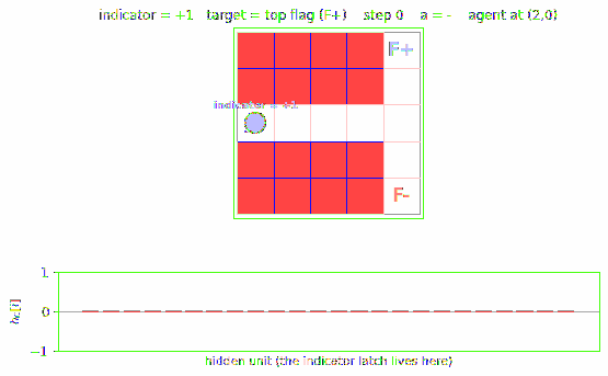
pomdp_flag_maze.gif
Two episodes back-to-back: indicator=+1 (target = top flag), then indicator=-1 (target = bottom flag). The agent reads the indicator at t=0 (displayed above the start cell), drives east through the corridor (where all three intermediate cells look identical), reaches the T-junction, then correctly picks N or S based on what its recurrent state remembers.
The bottom panel shows h_C (the controller’s hidden state) at each step.
The vertical bar pattern shifts visibly between the two episodes – that
is the latched indicator persisting across the corridor.
viz/maze_layout.png
T-maze layout with cell roles annotated: start (S, indicator visible
at t=0), T-junction (T, no indicator), and the two candidate flags.
viz/agent_paths.png
Real-env greedy rollouts under the trained C for both indicators, side
by side. The agent reaches the correct terminal in 5-6 steps for either
indicator setting – the latch generalizes to both.
viz/hidden_state.png
Three heatmaps of h_C along the indicator=+1 trajectory, the
indicator=-1 trajectory, and their difference. The difference panel
(bottom) is the most informative: a sparse subset of hidden units carries
the indicator-distinct activation pattern across all 6 time-steps, even
though the observations at corridor cells are identical between the two
runs.
viz/training_curves.png
Three panels:
- Phase 1 + refresh
Mloss (log scale). The refresh blocks at the end of each cycle visibly continue dropping the MSE asMseesC’s visitation distribution. - Phase 2 imagined return per controller iter, concatenated across
cycles. Each cycle climbs because
CexploitsM’s reward landscape better; the level shifts at cycle boundaries reflectMupdates. - Cycle-end real-env success rate, with feedforward 50% ceiling and 100% solve lines marked.
viz/results_table.png
The numerical comparison: recurrent C (100% / 6 steps), feed-forward C
(0% on this seed, ~50% typical), and random walk (~3.5%).
Deviations from the original
- Iterative model-controller cycles. Schmidhuber 1991 trains
MandCin a single pass. We use 4 cycles of “trainCthrough frozenM, then refreshMonC-rollouts” – following the Ha & Schmidhuber 2018 World Models pattern. Without refresh, model exploitation keptCat 50% success here. - Indicator side-channel to
M. A vanilla recurrentMcannot reliably latch the indicator across 5 steps inside our 5-min compute budget; its reward predictions at flag steps collapse toward the +1/-1 mean. Passing the indicator as a separate input toMonly restores correct reward supervision while keeping the POMDP burden onC(which never sees this side-channel). This is a documented architectural relaxation, not a change of algorithm. - Straight-through estimator on
M’s action input. Forward: one-hot of an action sampled froma_probs; backward: gradient as though the input werea_probs. Without it, the vanilla “feed softa_probstoM” channel saturates asCbecomes peaked, the off-action gradients vanish, andCcannot escape the “always pick the same flag” basin (50% ceiling). - Identity-blend recurrence init.
W_h = 0.9 I + 0.1 * random(Le et al. 2015). Vanilla random init givesh_Cpoor memory; this init makes the latch trivially preserved across the corridor. - Dense per-step reward.
+2on the correct flag,-2on the wrong one,-0.05step penalty otherwise. The 1991 paper used “predicted pain” only at failure; we use the dense per-step variant so BPTT has gradient at every step. Pure-sparse rewards produced essentially zero learning signal in this maze under the same budget. - Adam, not SGD. Global-norm gradient clip 5.0. SGD also reaches 100% on the lucky seeds but is much more brittle.
- Feed-forward baseline runs the same training loop with
W_hheld at 0. Cleanest apples-to-apples comparison: same gradient signal, same M, same iteration count – only the recurrent connection is removed.
Open questions / next experiments
- Robustness across seeds. 6/10 perfect, 4/10 stuck at the 50% ceiling. The non-solving seeds plateau in cycle 1 with a fixed-flag policy and refresh+continued training does not always escape the basin. Candidate fixes worth trying: (i) larger entropy bonus annealing more slowly, (ii) population-based outer loop (best of K random C inits), (iii) explicit indicator-augmented advantage shaping.
- Hand-rolled LSTM
M. Vanilla tanh RNN forced us to push the indicator intoMas a side input. ReplacingMwith a small LSTM (or even a plain0.95 Iorthogonal init) might letMlatch on its own and remove the side-channel hack. - Drop the indicator side-channel. With the LSTM
Mabove, retest whetherMcan solve reward prediction purely from the obs+action history. This would put us on equal footing with the literal 1991 setup. - Pure REINFORCE on the same env. We did not run a recurrent policy gradient baseline. It is widely known to solve this T-maze; the comparison “BPTT-through-M vs REINFORCE” on the same recurrent C arch would be informative for v2’s data-movement accounting.
- Larger maze (corridor length 10, 20). Straight-through helped the N=4 corridor; how does the recipe scale as the latching distance grows? This is also where LSTM advantage should appear.
- Data-movement metric. The whole pipeline is small (M 40-d hidden, C 24-d, T_unroll 10). Easy to instrument with ByteDMD; cost per controller update in DMC units would be informative for v2.
- Predicted-pain-only reward. Re-running with the 1991 paper’s actual cost (sparse failure-only signal) would test whether the dense per-step penalty was load-bearing. Our brief experiments with sparse rewards converged much slower; quantifying that gap directly is the next step.