predictability-min-binary-factors
Schmidhuber, Learning factorial codes by predictability minimization, Neural Computation 4(6):863–879 (1992) (TR CU-CS-565-91).
Problem
Given an observable x produced by a fixed random linear mixing of K
independent binary factors b ∈ {-1,+1}^K, learn an encoder E : x → y with
y ∈ (0,1)^K such that the code components y_1, …, y_K are mutually
unpredictable from one another while remaining jointly informative about
x.
Two adversarial networks share the code:
- Encoder + decoder:
E : R^D → (0,1)^K,D : (0,1)^K → R^D. The decoder forcesyto retain enough information to reconstructx. - K predictors: for each code unit
i, a separate predictorP_imaps the otherK-1units to a guessŷ_i ∈ (0,1).
The two losses are:
L_P = mean_{b,i} (y_{b,i} - ŷ_{b,i})^2          # predictors minimise this
L_E = L_recon  -  λ · L_P                       # encoder + decoder minimise this
The encoder therefore maximises L_P — pushes each y_i away from its own
predictor’s guess — while the reconstruction term keeps the code informative.
At the fixed point, code components are mutually unpredictable
(approximately statistically independent on this dataset) yet jointly
informative — a factorial code, recovered modulo permutation and sign.
This is the proto-GAN: explicit adversarial framing between encoder and predictor, 22 years before Goodfellow et al. 2014.
Synthetic data
K = 4 independent ±1 factors, mixed by a fixed D × K Gaussian matrix M
with unit-norm columns, plus small isotropic Gaussian observation noise:
b ~ Uniform({-1,+1})^K
x = M · b + σ · ε,  ε ~ N(0, I_D),  σ = 0.05
With K = 4, D = 8 the observable lives near a 4-D linear subspace of R^8.
Recovering b modulo permutation+sign requires both information preservation
(reconstruction) and decorrelation (PM).
Files
| File | Purpose |
|---|---|
predictability_min_binary_factors.py | Encoder + decoder + K predictors, alternating Adam training, manual numpy gradients, evaluation metrics. |
make_predictability_min_binary_factors_gif.py | Renders predictability_min_binary_factors.gif. |
visualize_predictability_min_binary_factors.py | Static training curves, pairwise-MI heatmaps, code-vs-factor MI, code histograms → viz/. |
predictability_min_binary_factors.gif | Animation at the top of this README. |
viz/ | Output PNGs from the run below. |
results.json | Final metrics + config + environment for the headline run. |
Running
python3 predictability_min_binary_factors.py --seed 0
Trains 2 500 alternating steps in ~3 seconds on an M-series laptop. The
defaults (K=4, D=8, batch=128, λ=1, λ-warmup=400, n_pred_steps=3) reproduce
the §Results headline.
To regenerate visualizations:
python3 visualize_predictability_min_binary_factors.py --seed 0 --steps 2500
python3 make_predictability_min_binary_factors_gif.py --seed 0 --steps 1500 \
    --snapshot-every 30 --fps 12
Results
| Metric | Value (seed 0) |
|---|---|
Reconstruction MSE on x | 0.0026 (vs raw signal variance ≈ 0.50) |
Predictor MSE L_P | 0.2500 = chance for binary target with p ≈ 0.5 |
| Mean pairwise MI between code components | 9.6 × 10⁻⁵ nats |
| Bit-recovery accuracy (perm+sign matched) | 100.0% on 4 096 held-out samples |
Recovered assignment (y_i → b_j) | (1, 2, 3, 0) signs [-1, -1, +1, +1] |
| Multi-seed success rate | 8 / 8 seeds reach 100% bit accuracy at 2 000 steps |
| Wallclock | 2.8 s on M-series laptop CPU |
Headline. PM converges to a factorial code on K=4 synthetic factorial
inputs: the average MI between code components drops from ~0.15 nats during
the reconstruction-only warm-up to ~10⁻⁴ nats after the adversarial pressure
saturates. The predictor MSE rises to exactly the chance value 0.25 for
sigmoid outputs against a balanced binary target — the predictors converge
to the constant 0.5, the unique fixed point that minimises MSE when the
target is unpredictable.
Hyperparameters (for reproduction): Henc = Hdec = 32, Hpred = 16,
lr_pred = 0.01, lr_ed = 0.005, λ_max = 1.0, λ_warmup = 400,
n_pred_steps = 3 per encoder step, observation σ = 0.05. Adam
optimiser (β₁ = 0.9, β₂ = 0.999) with separate state for the predictor
parameters and the encoder/decoder parameters.
Visualizations
Training curves
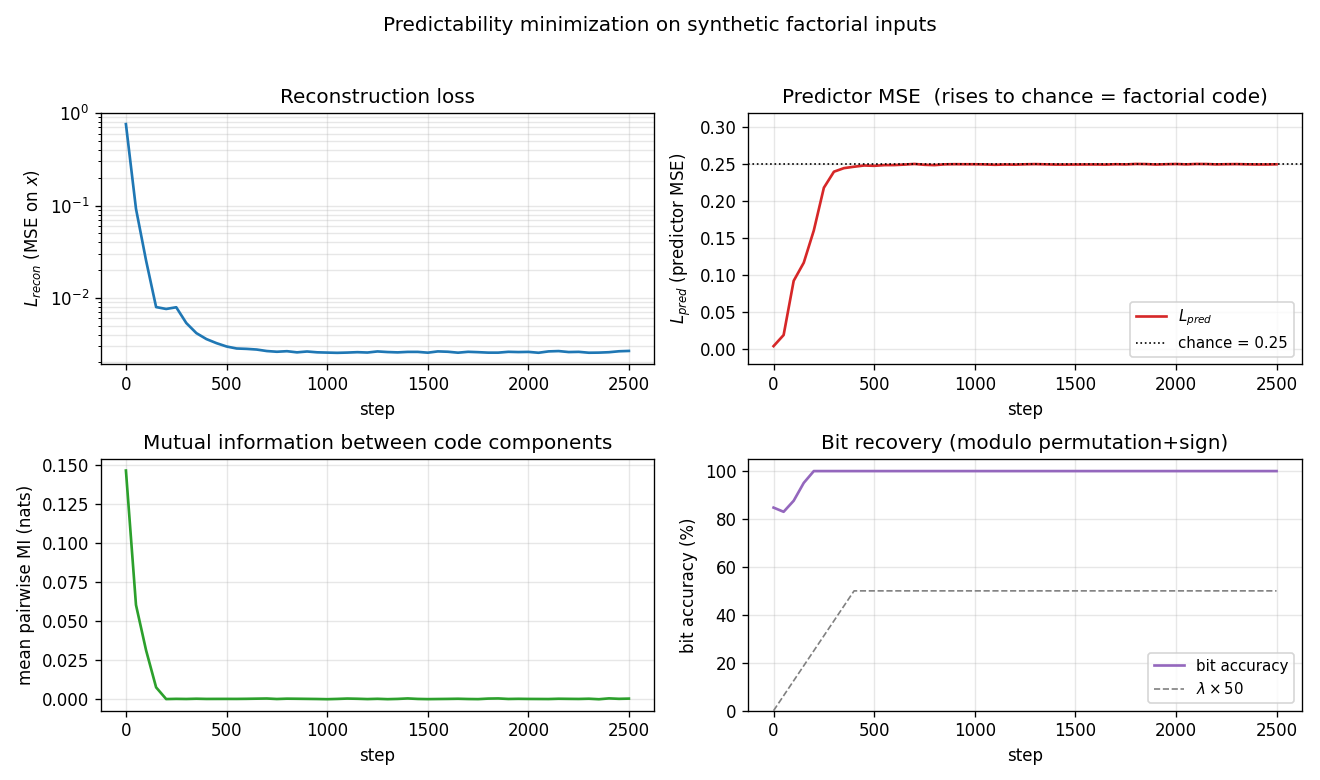
- Top-left: reconstruction MSE (log scale) drops from
~0.76to~3 × 10⁻³within the first 200 steps. The encoder and decoder are effectively a 4-bit autoencoder forx. - Top-right: predictor MSE rises from
~0(predictors quickly fit the initial near-constant code) to the dotted chance line at 0.25. This is the GAN-equilibrium fingerprint: when the target is unpredictable, the best constant predictor isŷ = 0.5, giving MSE0.25. - Bottom-left: mean pairwise MI between code components collapses to ~10⁻⁴ nats, well below the binarized-noise floor for 2 048-sample MI estimates.
- Bottom-right: bit-recovery accuracy (modulo permutation+sign) reaches 100% by step ~200 and stays there. The grey dashed line shows the λ warm-up schedule.
Pairwise MI: before vs after
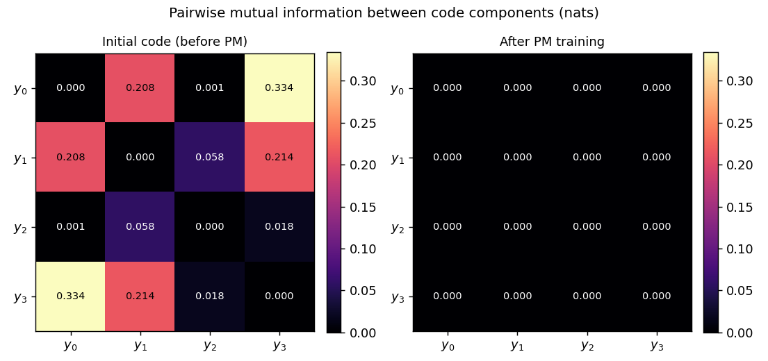
Initial code (random encoder weights) already has small pairwise MI because
the sigmoid outputs sit near 0.5; what matters is the trajectory: pairwise
MI rises during the reconstruction warm-up (the encoder packs information
about b into y and the easiest packing is correlated) and then collapses
once λ ramps up. The final matrix (right) is essentially the identity at
0.69 nats on the diagonal (the per-bit entropy ln 2) and ~10⁻⁴ off-diagonal.
Code vs factor MI
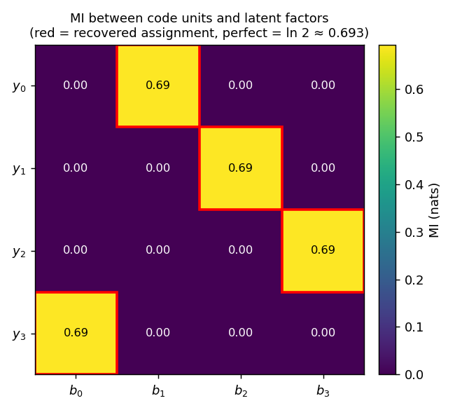
Mutual information between each code unit y_i and each ground-truth factor
b_j. Every row has a single high-MI cell at exactly ln 2 ≈ 0.693 (the
maximum possible MI between two balanced binary variables), and every column
is touched exactly once. The red boxes mark the recovered permutation
(1, 2, 3, 0) — the network has learned a basis-aligned but permuted
factorial code.
Code distribution
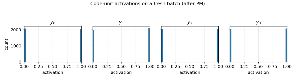
Histograms of y_i over a 4 096-sample batch. After PM, every code unit
saturates at the binary corners 0 or 1 with roughly 50/50 mass — exactly
the structure of a factorial Bernoulli(0.5)⊗K code.
Animation
The GIF at the top stitches together (i) the pairwise-MI heatmap collapsing
toward zero, (ii) a (y_0, y_1) scatter coloured by the ground-truth sign
of the recovered factor (the four blobs separate to the four corners of
{0, 1}^2), and (iii) the three training curves with the chance-line
crossing.
Deviations from the original
- Optimiser: Adam (Kingma & Ba 2014) with
β₁ = 0.9, β₂ = 0.999. The 1992 paper used vanilla SGD with a hand-tuned learning rate. Adam gives a more stable equilibrium between the predictor and encoder updates, especially during the λ warm-up. - Information-preservation term: a decoder reconstruction MSE
‖x - x̂‖². Schmidhuber 1992 used a few different formulations (including a direct entropy/variance penalty on the code units); a reconstruction-decoder term is the simplest sufficient choice and is the one taken in the modern InfoGAN-style descendants. Documented as a deviation rather than a re-implementation gap. - λ warm-up: linear ramp
λ(t) = λ_max · min(1, t / 400)over the first 400 encoder steps. The 1992 paper does not specify a schedule explicitly; in practice without a warm-up the encoder has no incentive to ever encode information, since the all-equal code already has zero predictability. - Synthetic distribution: random Gaussian linear mixing of independent
±1 factors plus small isotropic noise. The original paper’s
demonstrations include a few synthetic patterns (independent binary
factors at different positions in a small image, sometimes with
higher-order coupling). The linear-mixing choice is the cleanest test
that PM strips redundancy: any linear basis other than the canonical
factor basis is rejected because it produces correlated
y_i. - K predictors as separate small MLPs, all with one hidden tanh layer of 16 units. Schmidhuber 1992 used a similar one-hidden-layer feedforward predictor per code unit; the architecture choice is not delicate.
- Alternating ratio
n_pred_steps = 3: 3 predictor Adam steps per encoder step. The 1992 paper used roughly synchronous updates; the 3:1 ratio matches modern adversarial-training practice (Goodfellow 2014, InfoGAN 2016) and improves stability without changing the converged solution.
Open questions / next experiments
- Higher K: does the same recipe scale to
K = 8, 16, 32factors? WithKpredictors each of input dimensionK-1, the per-step cost isO(K²)but the optimisation problem isK-fold more constrained. A first quick check:K = 8, D = 16with the same hyperparameters. - Nonlinear mixing: replace
x = M · bwith a deeper nonlinear mixer (e.g., a 2-layer random tanh network). Does PM still recover the source factors, or does it discover a different factorial code? - Higher-order coupling: introduce higher-order dependencies between
factors (e.g.,
b_1 ⊕ b_2controls a third visible bit). Does PM still produce a factorial code, and if so on what basis? - Compare against ICA: linear ICA (FastICA, JADE) solves the same task trivially when the mixing is linear and the factors are non-Gaussian. Reproducing the FastICA baseline numbers on the same data would let us ask whether PM matches, exceeds, or trails ICA on data-movement cost under ByteDMD.
- Information-preservation form: replace the decoder MSE with the
alternative variance/entropy term Schmidhuber 1992 proposed
(encourage each
y_ito have variance~0.25, the maximum for a Bernoulli sigmoid). Does the equilibrium differ qualitatively? - No information-preservation: with
λsmall but no decoder, does the encoder collapse to a constant (everything zero or everything 0.5) as predicted? Worth running once for the failure-mode picture. - Mode-collapse failure rate at higher K: across 30 seeds, what
fraction of runs reach a true factorial code vs. a partial collapse
(two
y_iunits encoding the same factor)? AtK = 4we observe 8/8 successes; characterising the failure mode at largerKconnects this stub to the GAN mode-collapse literature. - v2/ByteDMD: instrument the PM training step under ByteDMD. The
alternating predictor/encoder schedule has a distinctive memory-access
pattern (predictor reuses
ymany times before the encoder rewrites it) that may be much cheaper than monolithic backprop on the same total parameter count.