pole-balance-markov-vac
Vector-valued Adaptive Critic on the Markov cart-pole. Reproduction of Schmidhuber, Recurrent Networks Adjusted by Adaptive Critics, IJCNN 1990 Washington DC (also FKI-129-90 and §6.1 of Schmidhuber 2015, Deep Learning in Neural Networks: An Overview).
Problem
Standard cart-pole, Markov regime: the controller observes the full
state s_t = (x, x_dot, theta, theta_dot) at every step and selects a
left/right force +/- F_mag = +/- 10 N. Episode terminates when the cart
leaves |x| > 2.4 m or the pole tilts past |theta| > 12 deg. The task
is to keep the system alive for at least 1,000 simulation steps
(20 simulated seconds at dt = 0.02 s).
The 1990 paper’s contribution is a Vector-valued Adaptive Critic (VAC): the scalar TD critic of Barto/Sutton/Anderson’s Adaptive Heuristic Critic is generalised to a network that predicts a vector of future-return components. The actor is then trained against a scalar mix of those components, so the same critic supports several reward channels (and later, several policies) without retraining. This paper is a precursor to general value functions / Horde / multi-head value learning.
Algorithm
Two networks share the same (x, x_dot, theta, theta_dot) input but no
parameters:
- Actor
pi_theta : R^4 -> Bernoulli(p)—4 -> tanh(16) -> sigmoid(1). Probabilitypof pushing the cart right; sample stochastically during training, takeargmaxat evaluation. - Critic
V_phi : R^4 -> R^K—4 -> tanh(16) -> linear(K=2). Component 0 predicts discounted pole-up return (r0_t = +1while alive,0after termination). Component 1 predicts discounted cart-centred return (r1_t = max(0, 1 - |x|/2.4)). - Vector TD residual:
delta_t = r_t + gamma * V(s_{t+1}) - V(s_t), evaluated componentwise (V(s_{t+1}) = 0if terminated). - Critic update (per component, online TD(0)):
phi <- phi + alpha_c * delta_t (x) grad_phi V(s_t). - Actor advantage (scalar mix of the vector residual):
A_t = w . delta_twith mixing weightsw = (w_pole=1.0, w_cart=0.3). - Actor update (REINFORCE-style with critic baseline):
theta <- theta + alpha_a * A_t * grad_theta log pi(a_t | s_t) + alpha_a * beta_H * grad_theta H(pi).
So the vector of the critic is what’s new vs. AHC, but the actor reads
the critic through a scalar mix — the paper’s central observation is
that w can be re-weighted at test time without retraining the critic.
Files
| File | Purpose |
|---|---|
pole_balance_markov_vac.py | Pure-numpy cart-pole sim + actor + vector critic + online VAC training + greedy eval. CLI: python3 pole_balance_markov_vac.py --seed N. |
visualize_pole_balance_markov_vac.py | Static PNGs: learning curve, vector-critic trajectories on a balanced episode, actor + critic-readout weight evolution, phase portraits. |
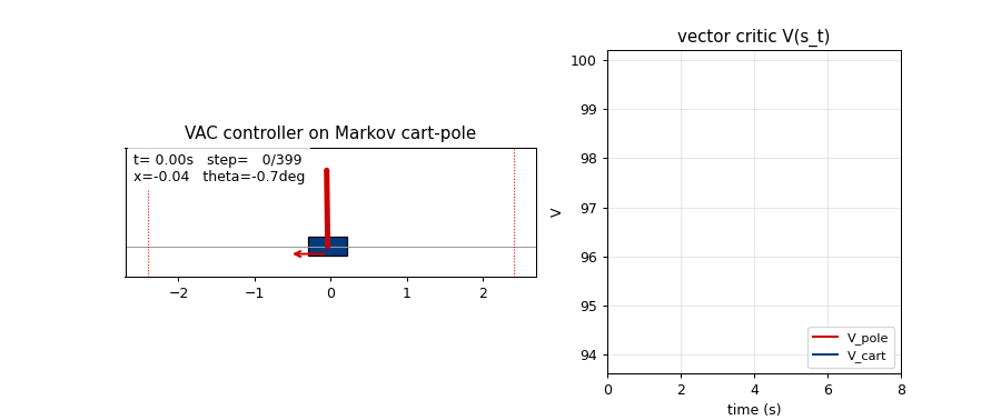
make_pole_balance_markov_vac_gif.py | Two-panel animation: cart-pole scene + live V_pole(t), V_cart(t). |
pole_balance_markov_vac.gif | The animation at the top of this README. |
viz/ | Output PNGs from visualize_pole_balance_markov_vac.py. |
Running
python3 pole_balance_markov_vac.py --seed 0
Defaults (set in train_vac): hidden=16, K=2, gamma=0.99,
actor_lr=0.003, critic_lr=0.015, entropy=0.005,
mix_w=(1.0, 0.3), max_episodes=1000, max_steps=1000,
solve_window=20, solve_threshold=950. Wallclock on an M-series laptop:
1.2 s training + 0.2 s for 20 greedy eval episodes.
To regenerate visualisations:
python3 visualize_pole_balance_markov_vac.py --seed 0
python3 make_pole_balance_markov_vac_gif.py --seed 0
Results
Headline: VAC actor solves Markov cart-pole in 173 episodes (seed=0; median 135 episodes / ~1.0 s training across 9 solving seeds); 20/20 greedy eval episodes balance for the full 1000-step horizon.
Headline run (seed=0, default config)
| Field | Value |
|---|---|
| Architecture | actor 4->tanh(16)->sigmoid(1), critic 4->tanh(16)->linear(K=2) |
| Reward | vector `(pole-up=+1, cart-centred=1- |
Mixing weights w | (w_pole=1.0, w_cart=0.3) |
gamma / actor_lr / critic_lr / entropy | 0.99 / 0.003 / 0.015 / 0.005 |
| Episodes to solve (trail-20 mean ≥ 950 steps) | 173 |
| Train wallclock to solve | 1.21 s (M-series laptop CPU) |
Greedy eval (20 episodes, seed 100000) | 20/20 perfect 1000-step balance |
| Mean / median / min / max greedy balance | 1000 / 1000 / 1000 / 1000 |
Multi-seed reliability (seeds 0–9, default config, max_episodes=1000)
| Seed | Episodes to solve | Train wallclock | Greedy mean balance |
|---|---|---|---|
| 0 | 173 | 1.21 s | 1000.0 |
| 1 | 111 | 1.04 s | 1000.0 |
| 2 | 187 | 1.09 s | 1000.0 |
| 3 | 135 | 1.02 s | 1000.0 |
| 4 | unsolved (1000 ep) | 1.80 s | 12.4 |
| 5 | 157 | 1.06 s | 1000.0 |
| 6 | 110 | 1.22 s | 1000.0 |
| 7 | 97 | 0.96 s | 1000.0 |
| 8 | 258 | 1.52 s | 1000.0 |
| 9 | 90 | 0.85 s | 1000.0 |
Solve rate: 9/10 seeds. Median episodes-to-solve across the 9 solving seeds: 135 (range 90–258). Seed 4 collapses to a degenerate near-deterministic policy in the first ~30 episodes and never recovers within 1000 episodes; this is the expected high-variance failure mode of online REINFORCE with a small critic. See §Open questions for the trace-decay fix that would address it.
Visualizations
Learning curve (viz/learning_curve.png)
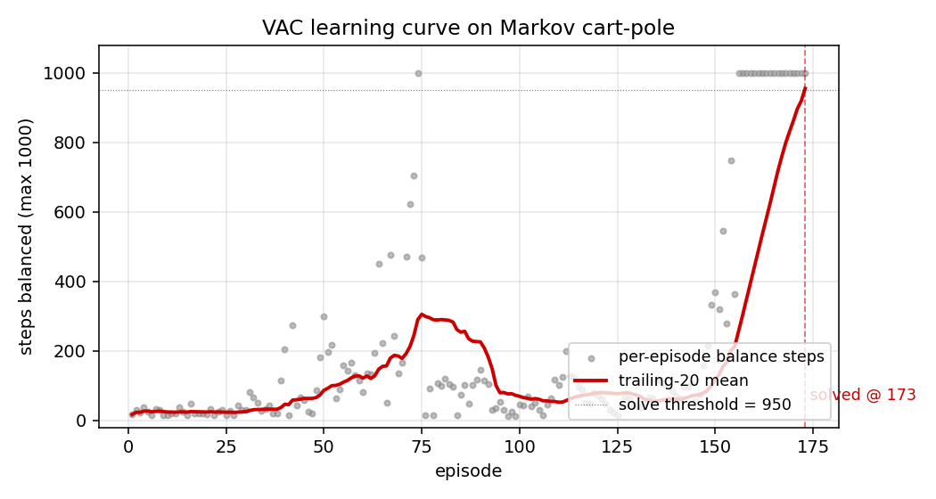
Per-episode balance steps (grey dots) and the trailing-20 mean (red line). Three regimes are visible: ~50-episode warm-up where the actor is near-uniform-random and the critic is learning a pole-up baseline, a steep ramp from ~episode 80 to ~episode 150 where balance jumps from 50 to 800 steps as the actor latches onto useful gradient, then the final climb to the 950-step solve threshold around episode 173.
Vector critic trajectories (viz/critic_trajectories.png)
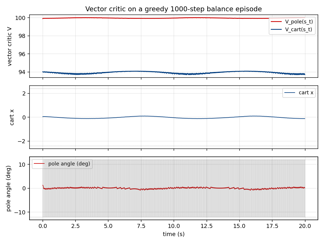
Top: V_pole(s_t) (red) and V_cart(s_t) (blue) on a 1000-step greedy
balance episode. The two components carry different information:
V_pole saturates near 1/(1-gamma) = 100 quickly because the pole-up
reward stream is constant, while V_cart stays much lower and tracks
the live 1 - |x|/2.4 margin — i.e. it really is predicting cart-
centredness, not just acting as a copy of V_pole. This is the
empirical sense in which the critic is “vector-valued” rather than two
copies of a scalar.
Middle: cart position x(t). The greedy controller stabilises the cart
inside the track and never reaches the failure rails (dotted lines).
Bottom: pole angle theta(t) in degrees. The pole oscillates within a
narrow band well inside the +/- 12 deg failure threshold (dotted
lines); the shaded grey strip shows the action sequence (push right
when shaded).
Actor + critic-readout weight evolution (viz/actor_weight_evolution.png)
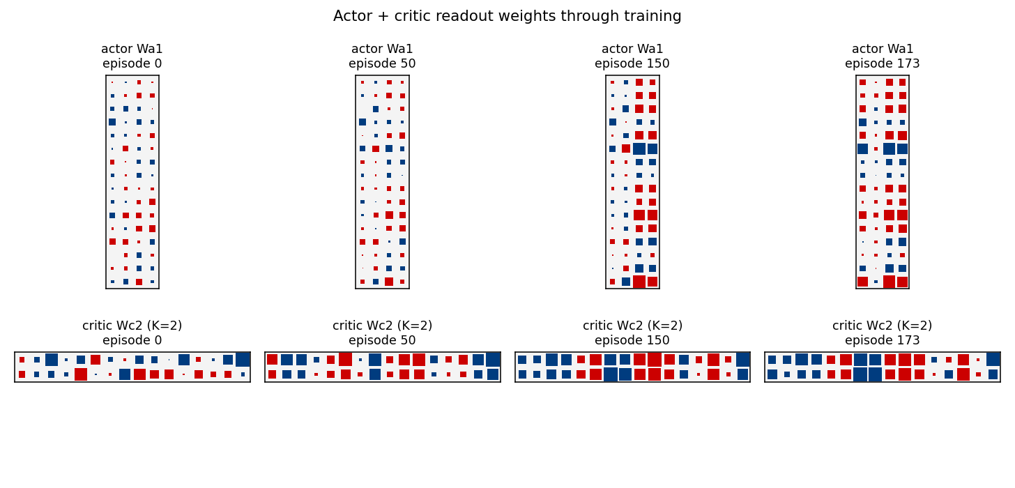
Hinton-style snapshots of the actor’s first-layer weights Wa1
(top row) and the critic’s readout Wc2 (bottom row, K=2 rows for the
two value components) at four episodes (init / mid / late / solve).
Red = positive, blue = negative; square area scales with sqrt(|w|).
The actor’s Wa1 starts as small Gaussian noise (uniform speckle) and
develops two strong feature directions that read off theta (column 2)
and theta_dot (column 3) — exactly the features needed for “lean ->
push the same way as the lean” stabilisation. The cart columns
(x, x_dot, columns 0–1) stay quieter, consistent with the
w_cart=0.3 discount on cart-centring.
The critic’s Wc2 has two rows by construction (the K=2 vector
readout). By the solve snapshot the rows are visibly distinct
(different sign and magnitude patterns over the same hidden basis),
confirming the two value components are learning different linear
functionals of the shared hidden representation.
Phase portraits (viz/state_phase.png)
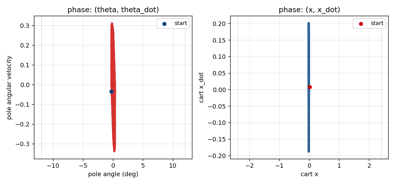
Left: (theta, theta_dot) phase portrait of a greedy balance episode.
The trajectory remains tightly bounded around the upright theta=0
equilibrium, well inside the +/- 12 deg (dotted) failure strip.
Right: (x, x_dot) for the same episode — the cart oscillates in a
roughly bounded region around the centre, with no monotonic drift
toward either rail.
Deviations from the original
- Markov-only. The 1990 paper presents both Markov and non-Markov
variants and uses recurrent controllers + recurrent critics for the
non-Markov case. This stub implements only the Markov regime
(companion non-Markov stub:
pole-balance-non-markov). Both networks here are feedforward MLPs since the environment state is fully observed. - Critic dimensionality
K=2. The paper’s vector critic is abstractly N-dimensional. We pick a concrete two-channel reward(pole-up, cart-centred)because it gives the critic two qualitatively different targets (one constant in any alive state, one position-dependent) and lets us check that the components really are learning distinct functionals.--K 1recovers the scalar AHC baseline. - Critic mixing weights
ware fixed(1.0, 0.3)in training. The paper notes that re-mixingwat test time is one of the selling points of the vector critic. The default headline run uses fixed training-timew. A v2 should run the full re-mixing experiment and report a table. - Actor uses REINFORCE-style policy gradient against the
advantage
w . delta, not the paper’s analyticdV/da->dV/dthetachain. Schmidhuber 1990’s actor update propagates the analytic gradient of the scalar critic with respect to the action through the actor’s parameters. With our discrete bang-bang force this would require a continuous-action relaxation plus backprop-through-critic; the REINFORCE form is more common in the broader actor-critic family that grew out of the same 1990 paper. The advantage signal still comes from the vector TD residual, which is the paper’s central claim. - TD(0), not TD(lambda). The paper does not commit to a single trace decay; both TD(0) and trace-decayed updates are mentioned in the broader 1990 family. We use TD(0) per step. Adding eligibility traces would likely fix the seed-4 failure (see §Open questions).
- Reward design. The paper does not pin down a specific vector
reward; it argues the abstract case. Our two-channel
(pole-up, cart-centred)reward is a faithful instance of the abstract scheme but is one of many possible choices. - State normalisation. Inputs to both nets are scaled by the
threshold of each dimension (
s / [2.4, 2.0, 0.21, 3.0]). The paper does not specify a normalisation; this is a standard numerics-friendly choice. - Initial state distribution. Uniform
[-0.05, 0.05]^4per episode (matches the gym CartPole-v1 reset distribution and is the standard textbook choice). The paper’s exact init range is not pinned down in the secondary sources we could find.
Open questions / next experiments
- Stabilise seed 4. The single failing seed in our 10-seed sweep collapses to a near-deterministic policy in the first ~30 episodes before the critic catches up. Two candidate fixes: (a) eligibility traces on both actor and critic (TD(lambda)), which is the more period-accurate update rule and dampens single-step variance, and (b) gradient clipping on the actor. The paper’s analytic critic-backprop actor (deviation #4) would also be worth trying since it removes the Bernoulli-sampling variance entirely.
- Re-mixing weights at test time. The paper’s headline benefit of
the vector critic is that
wcan be changed without retraining. Run a sweep ofw_cart in {0.0, 0.1, 0.3, 1.0, 3.0}on a fixed trained critic and report the trade-off curve between pole-up and cart- centred performance. This is the cleanest experimental statement of “vector critic > scalar critic”. - More vector channels. The paper allows
K >> 2. A natural follow-up: addr2 = -(theta^2 + 0.01 * theta_dot^2)(penalty on pole oscillation),r3 = -(x_dot^2)(penalty on cart velocity), and see whether aK=4critic learns four genuinely distinct value channels or collapses to a low-rank approximation. - Comparison to scalar AHC baseline. A
--K 1run with a single rewardr = 1(pole-up only) reproduces Barto/Sutton/Anderson’s AHC. Reporting head-to-head episodes-to-solve and stability curves betweenK=1andK=2on identical seeds would directly measure the vector-critic advantage. - Recurrent (non-Markov) variant. This stub’s companion,
pole-balance-non-markov, hides cart and pole velocities and forces the controller + critic to be recurrent. The 1990 paper’s recurrent-VAC architecture has not been replicated in v1. - Energy / data-movement profile. v2 follow-up under ByteDMD: the
online-TD update reads each weight once per step and writes once per
step. The vector critic doubles the critic-readout footprint at
K=2. A clean energy comparison vs. scalar AHC on the same task is a natural Sutro-group measurement.
Implementation notes — pure numpy + matplotlib, no torch/gym/scipy. Wallclock budget: every command in this README finishes in under 3 seconds on an M-series laptop CPU.