Visual tour

Yad's wave-build swarms reproduced two catalogs of papers as runnable stubs, each one committing a training animation. All 111 are below in catalog order, every card tracing back to a paper and a folder of code. The GIFs stream from each catalog's own pages.

hinton-problems 54 source tour

Geoffrey Hinton's catalog, 1985 to 2022, as runnable stubs.

1980s, Connectionist foundations

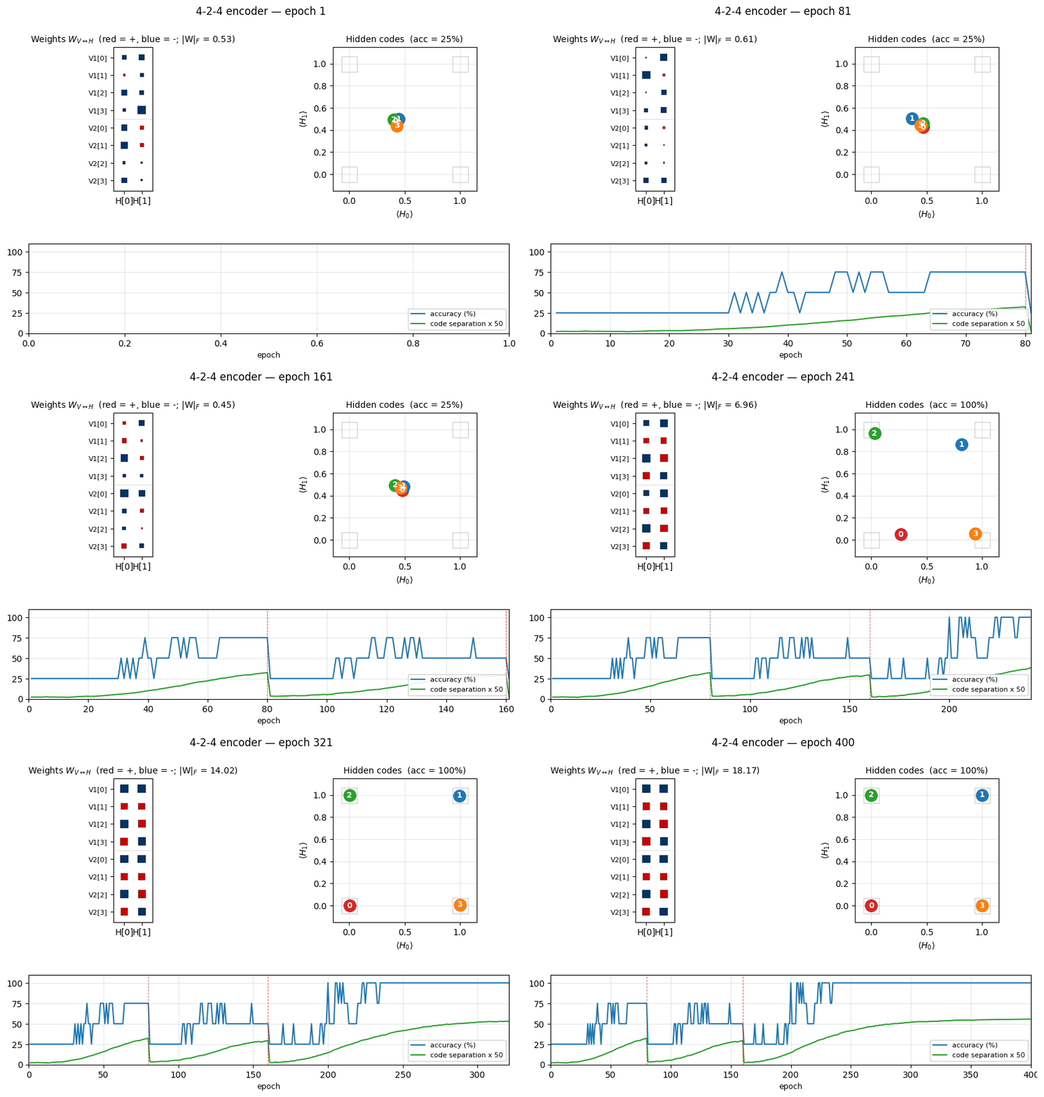
encoder-4-2-4 — ★ encoder-4-2-4 Ackley, Hinton & Sejnowski (1985), A learning algorithm for Boltzmann machines Two groups of 4 visible binary units (V1, V2) connected through 2 hidden binary units. The bottleneck has exactly log2(4) bits of capacity, so the only correct solution puts the 4 training patterns on the 4 corners of {0, 1}^2.

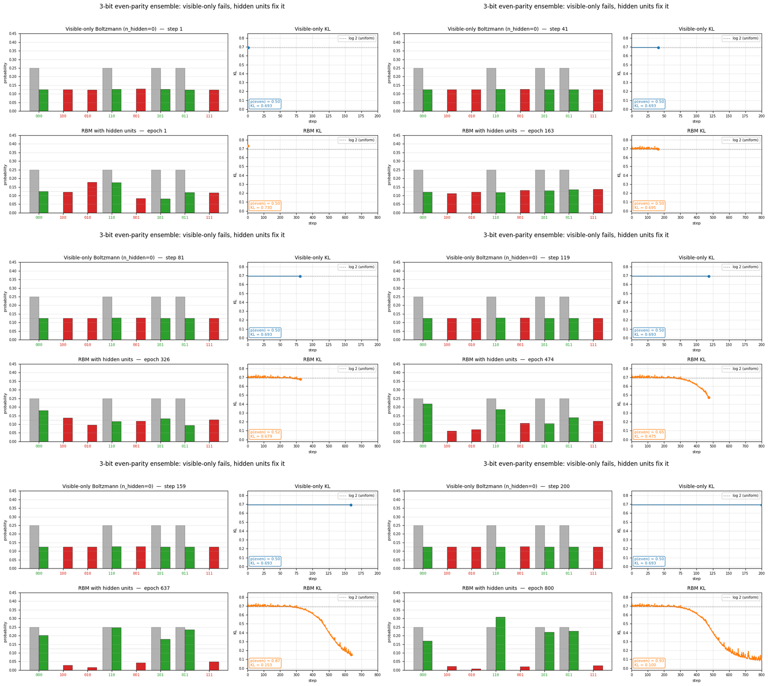
encoder-3-parity — encoder-3-parity Ackley, Hinton & Sejnowski (1985), A learning algorithm for Boltzmann machines 3-bit even-parity. The point of this stub is the visible-only Boltzmann hits a hard floor of KL = log 2 ≈ 0.693 (it can only memorize even-cardinality marginals);

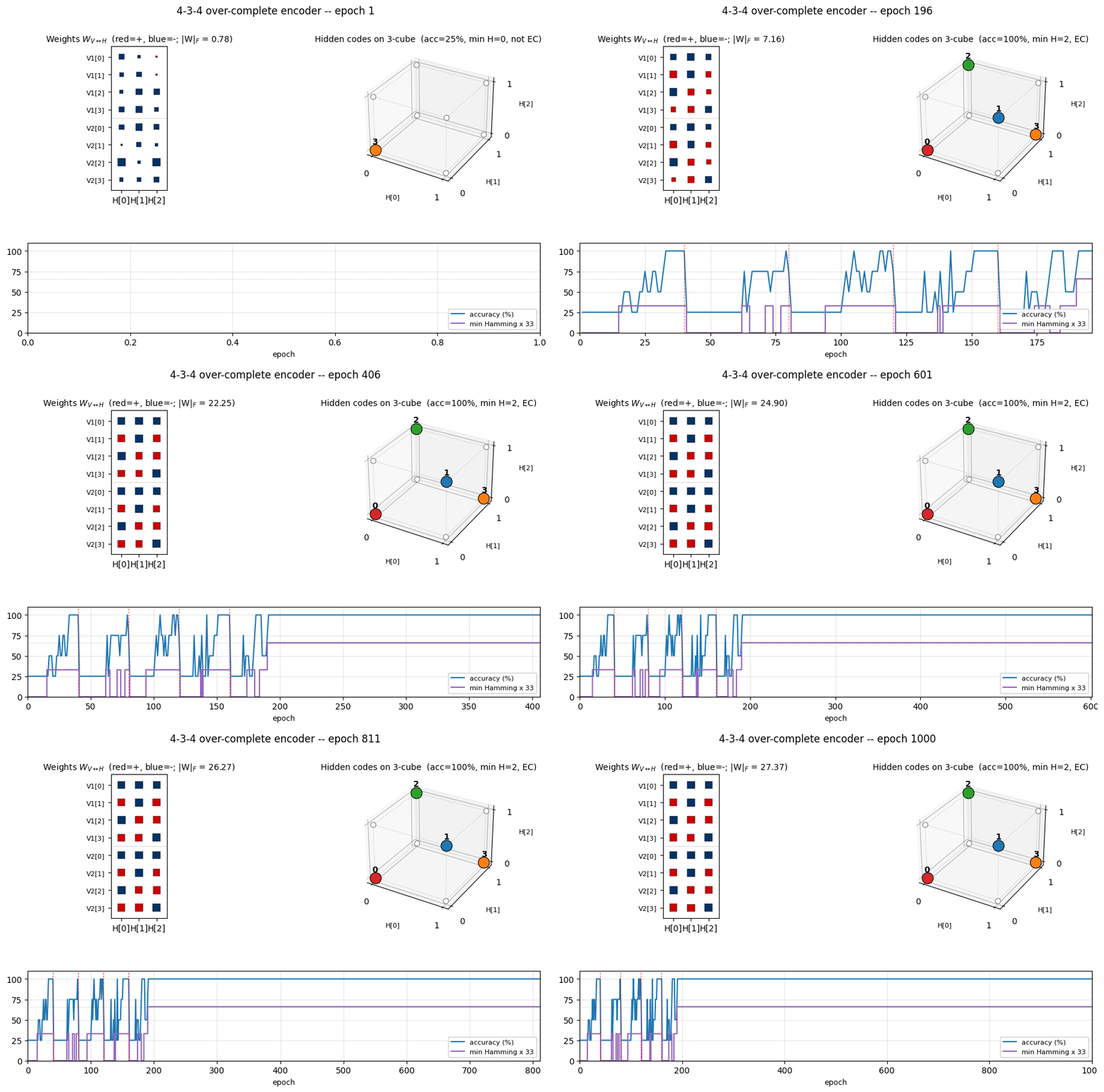
encoder-4-3-4 — encoder-4-3-4 Ackley, Hinton & Sejnowski (1985), A learning algorithm for Boltzmann machines Over-complete encoder, 3 hidden bits to encode 4 patterns, leaving room for an error-correcting code to emerge. At the right seed the network finds the even-parity codeset (Hamming distance ≥ 2 between any two codes);

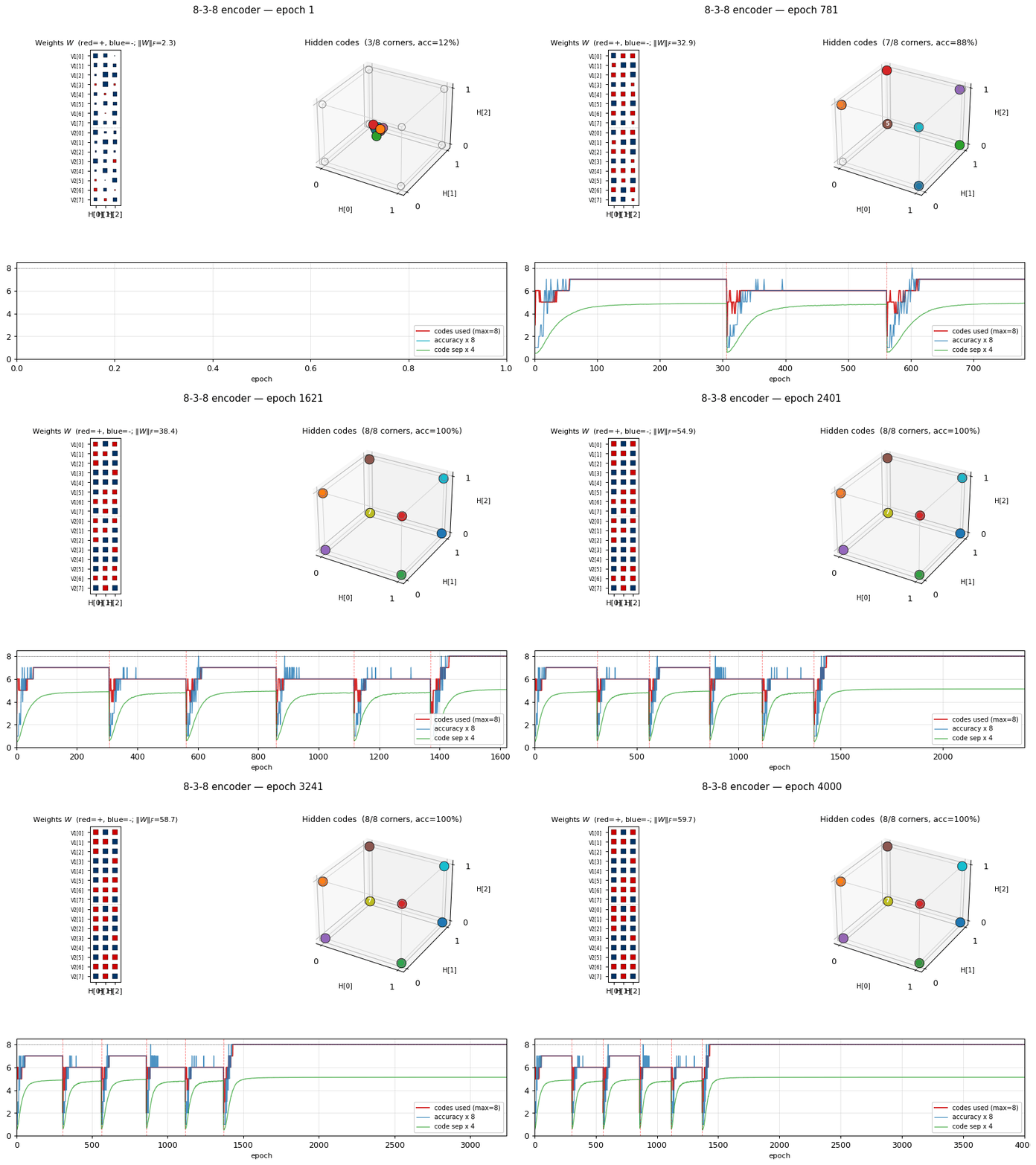
encoder-8-3-8 — encoder-8-3-8 Ackley, Hinton & Sejnowski (1985), A learning algorithm for Boltzmann machines The information-theoretic minimum: 8 patterns through 3 hidden bits (log2(8) = 3). Hits the paper's reported 16/20 success rate exactly. GIF tracks the 8 hidden codes spreading to the 8 corners of {0, 1}^3.

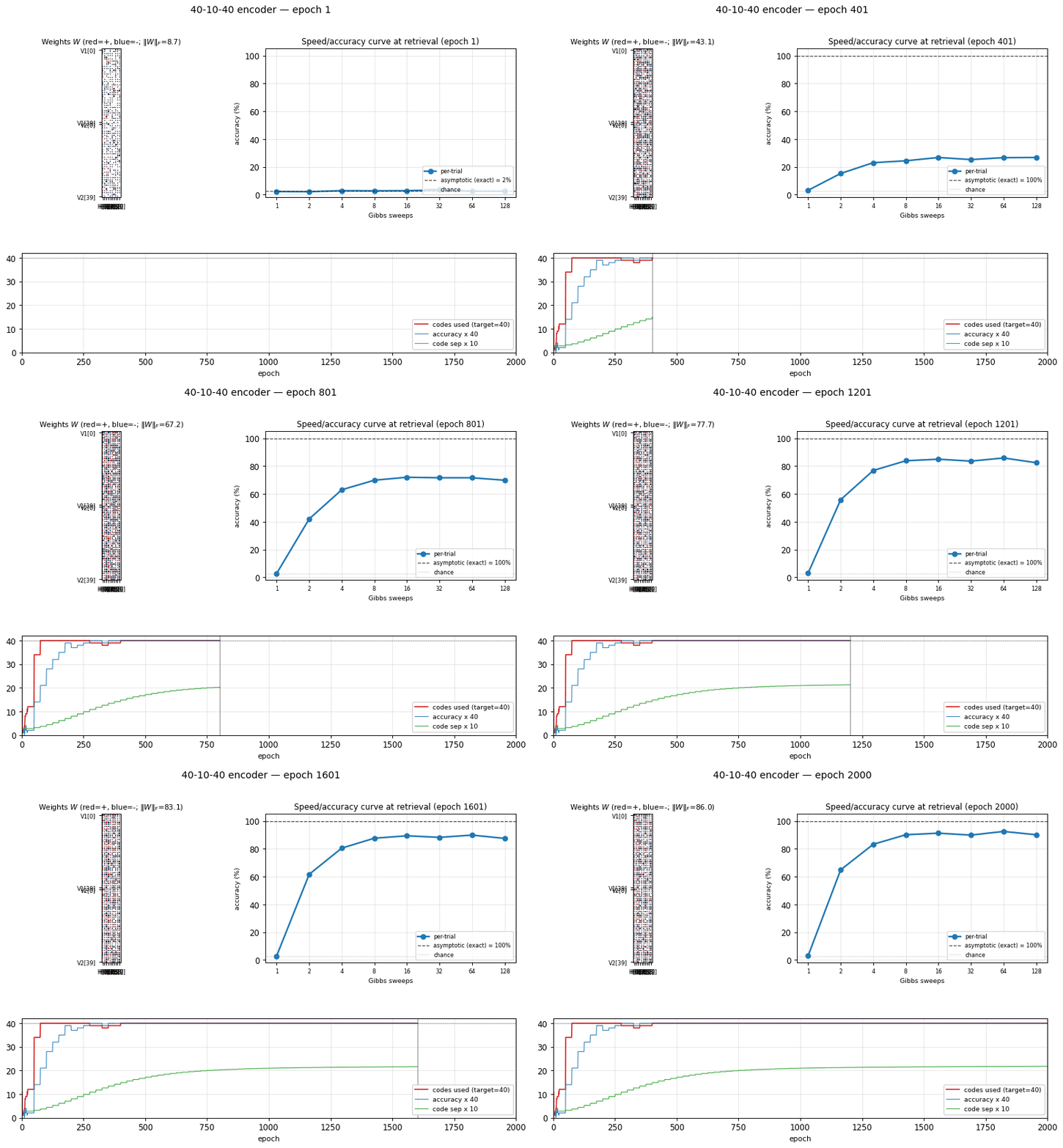
encoder-40-10-40 — encoder-40-10-40 Ackley, Hinton & Sejnowski (1985), A learning algorithm for Boltzmann machines Scale stress-test of the same recipe. With 40 patterns through 10 hidden bits the local-minima problem softens (lots of valid codes) and CD-k recovers cleanly, modern sampling actually beats the 1985 simulated- annealing number.

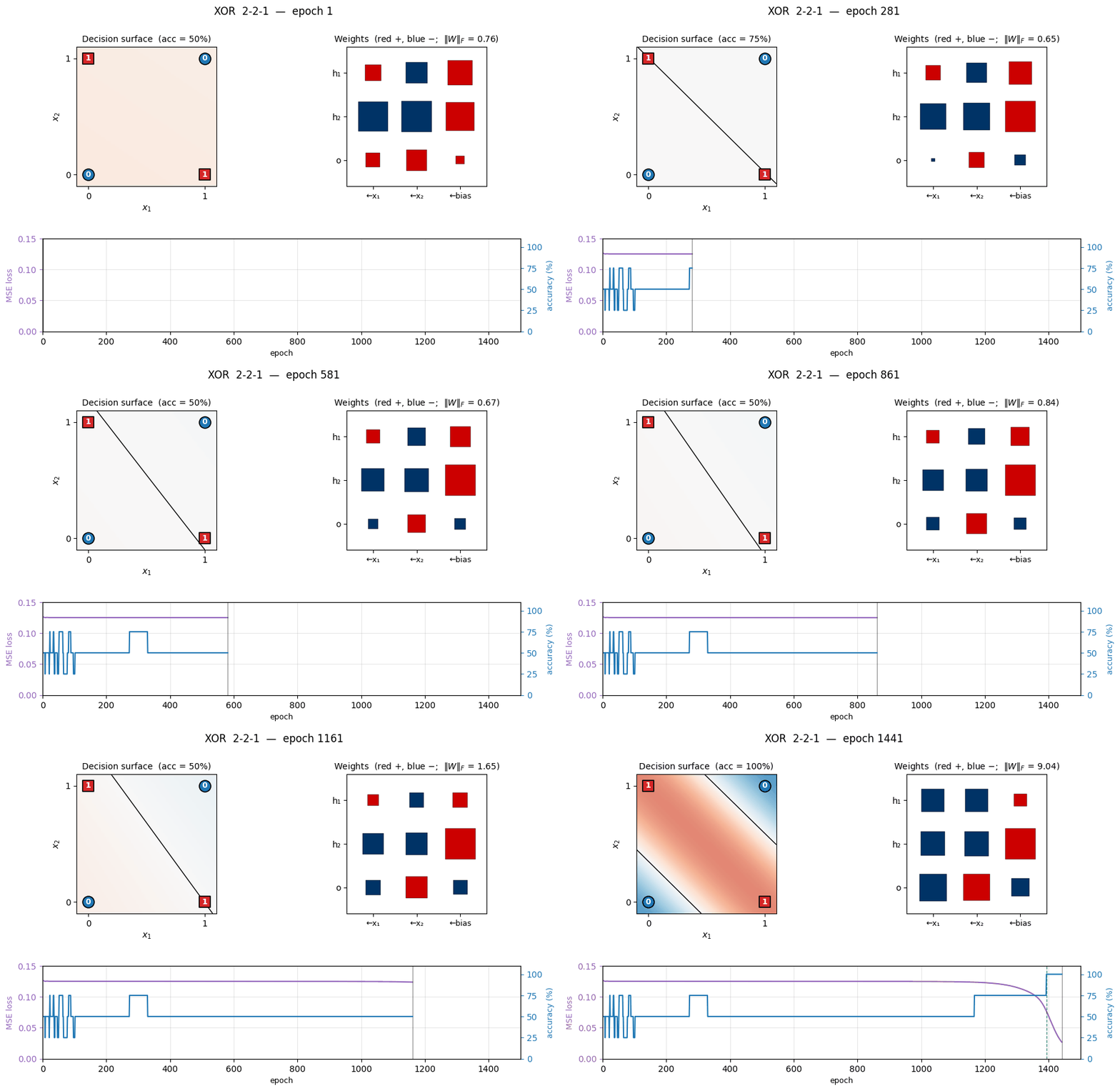
xor — xor Rumelhart, Hinton & Williams (1986), Learning internal representations by error propagation The canonical 2-bit XOR. The decision-surface panel shows the network slicing the unit square along the anti-diagonal once the hidden layer has shaped two well-placed half-planes.

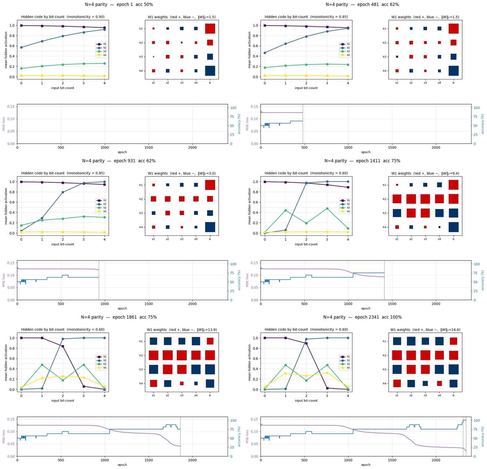
n-bit-parity — n-bit-parity Rumelhart, Hinton & Williams (1986), Learning internal representations by error propagation Generalization of XOR to N bits. Thermometer-coded hidden units can be seen forming as N grows; the difficulty scales as advertised.

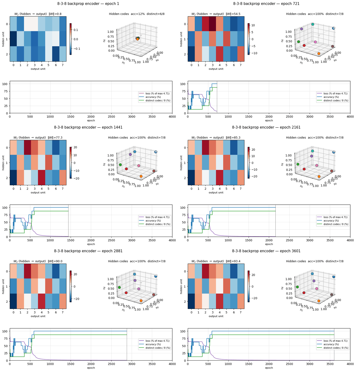
encoder-backprop-8-3-8 — encoder-backprop-8-3-8 Rumelhart, Hinton & Williams (1986), Learning internal representations by error propagation The backprop counterpart to the Boltzmann encoder above. Same problem, different gradient, and 70% of seeds reach exactly 8 distinct hidden codes. Useful side-by-side with encoder-8-3-8 to see what the sampling/temperature schedule buys you.

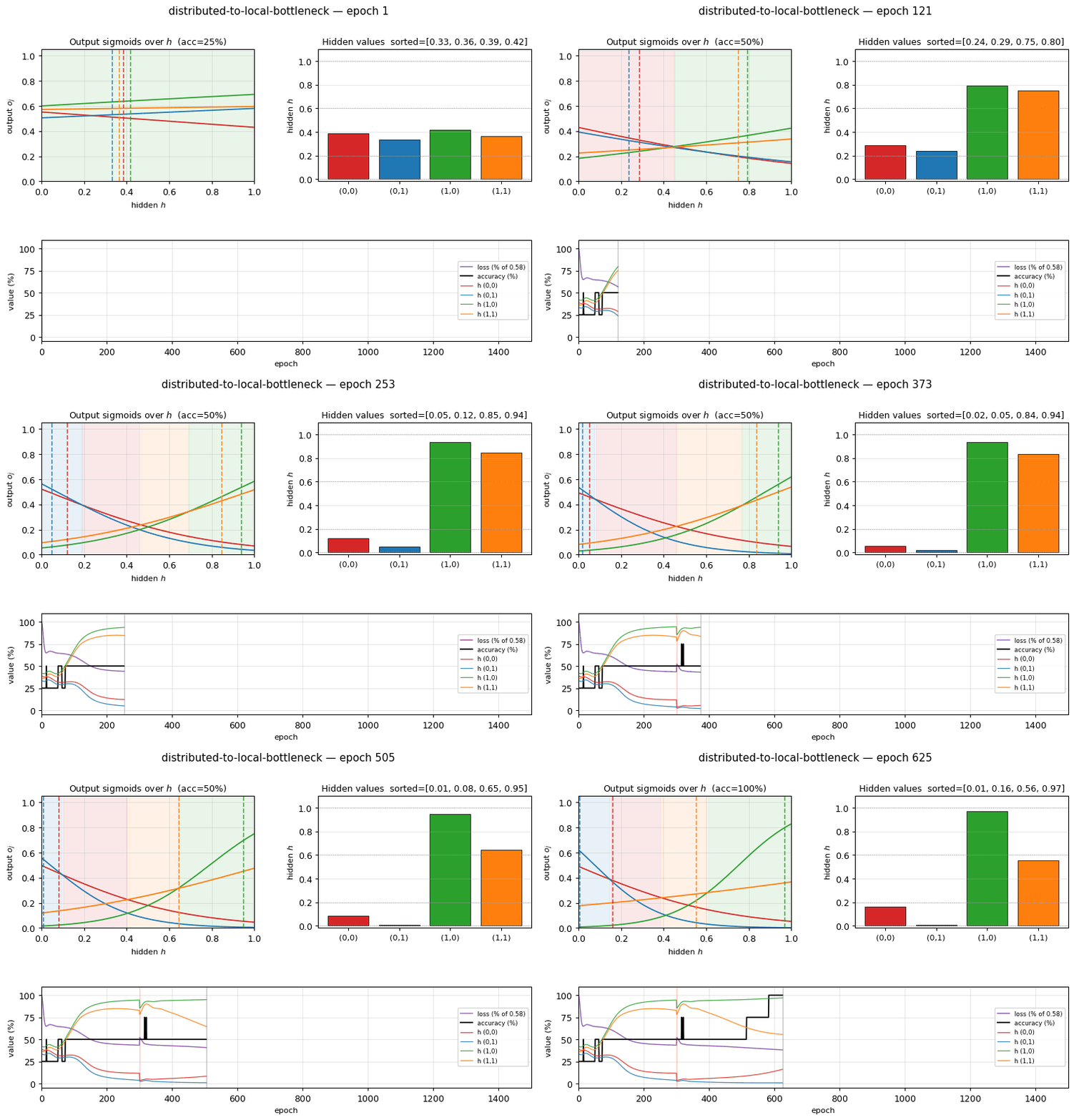
distributed-to-local-bottleneck — distributed-to-local-bottleneck Rumelhart, Hinton & Williams (1986), Learning internal representations by error propagation Smallest example of a graded single-unit code. One hidden unit must output 4 distinct real values to encode 4 patterns. The animation watches those values pull apart along the unit interval, paper reported (0, 0.2, 0.6, 1.0);

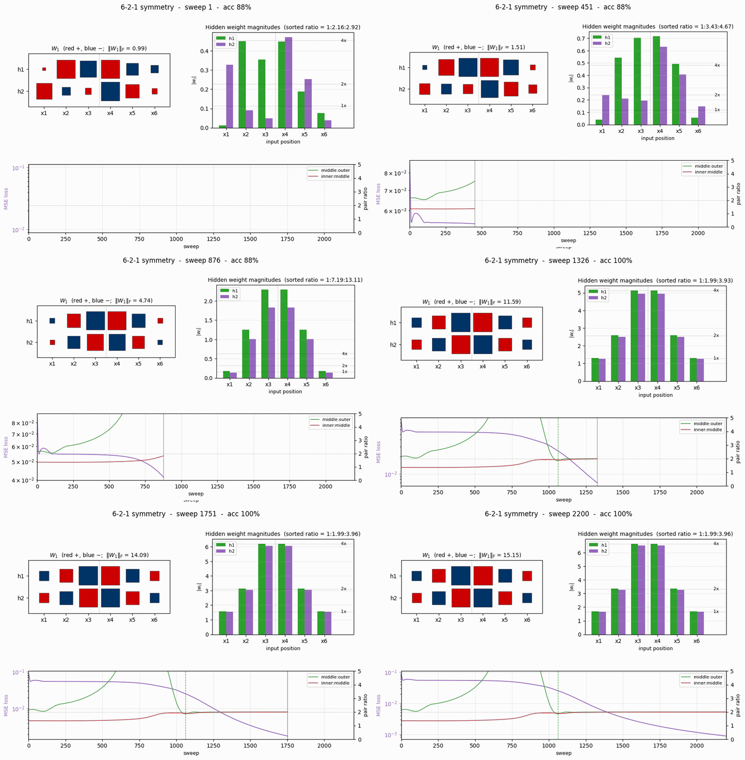
symmetry — symmetry Rumelhart, Hinton & Williams (1986), Learning internal representations by error propagation 6-bit palindrome detection from a single hidden unit. The famous 1 : 2 : 4 antisymmetric weight pattern falls out automatically; the weight Hinton diagram makes the geometric-progression pattern visible by eye at convergence.

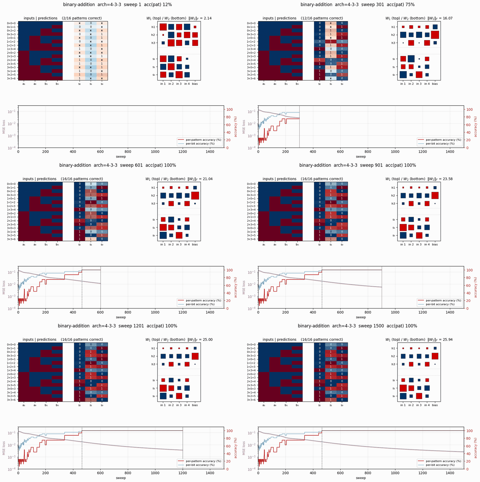
binary-addition — binary-addition Rumelhart, Hinton & Williams (1986), Learning internal representations by error propagation Two 2-bit numbers in, 3-bit sum out. The interesting story is the local-minima study: a 4-3-3 network solves it; the bottlenecked 4-2-3 network cannot, the 2-hidden-unit version provably does not have enough capacity to disentangle carry from value.

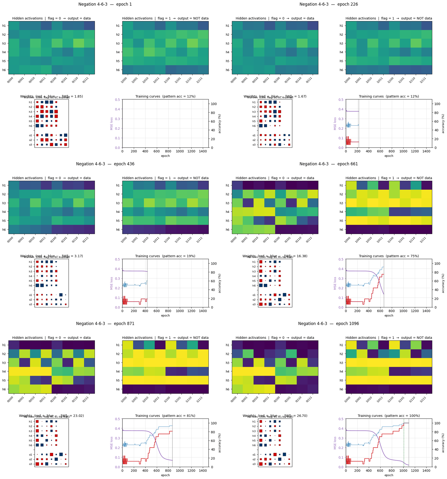
negation — negation Rumelhart, Hinton & Williams (1986), Learning internal representations by error propagation Flag-conditioned bit-flip, one input flag controls whether the other inputs are passed through or flipped.

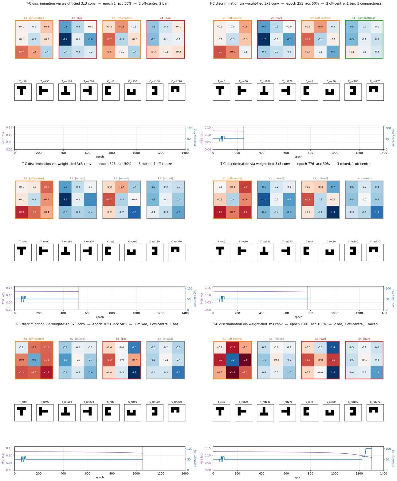
t-c-discrimination — t-c-discrimination Rumelhart, Hinton & Williams (1986), Learning internal representations by error propagation Shared-weight retina discriminating T from C across translations. With weight-tying across spatial positions (the 1986 ancestor of convolutions) the network grows three families of detectors, corner, edge, and T-junction, visible in the kernel.

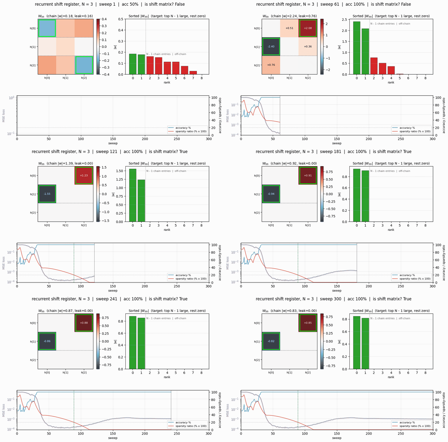
recurrent-shift-register — recurrent-shift-register Rumelhart, Hinton & Williams (1986), Learning internal representations by error propagation An RNN learning to be a pure shift register. Both N=3 and N=5 well under the paper's <200-sweep threshold. GIF shows the recurrent state walking through its cycle in lock-step with the input.

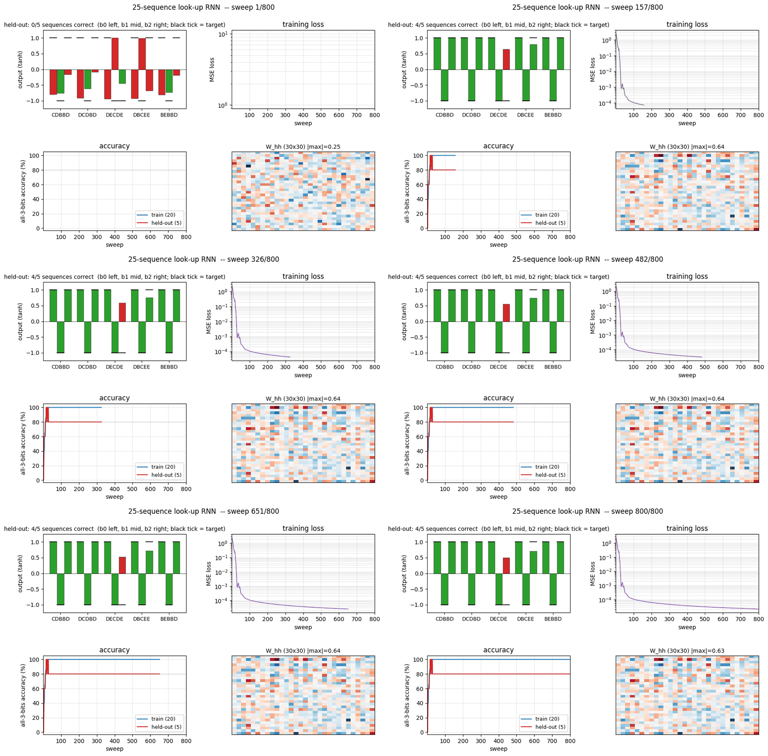
sequence-lookup-25 — sequence-lookup-25 Rumelhart, Hinton & Williams (1986), Learning internal representations by error propagation A small RNN learning to retrieve which of 25 stored sequences matches a prefix. The viz folder is the largest in the repo (12 PNGs), per-task attention traces and per-position retrieval curves are worth a look.

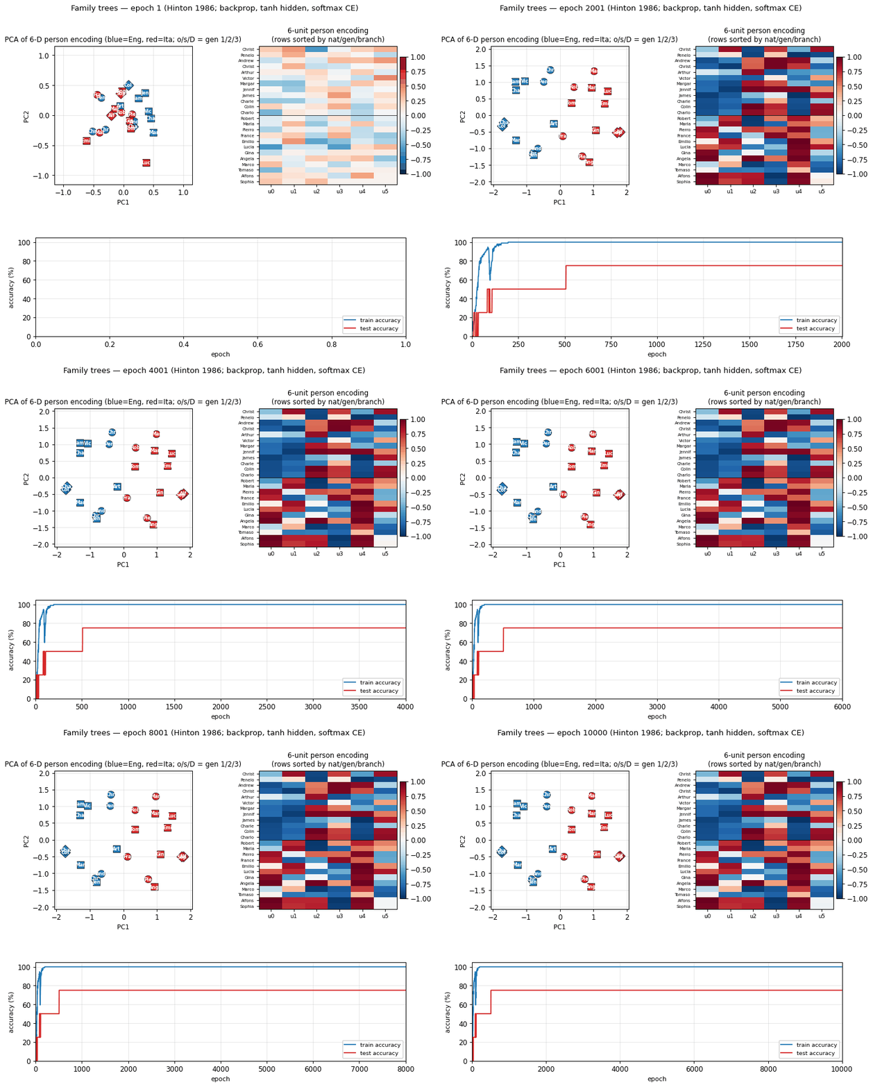
family-trees — family-trees Hinton (1986), Learning distributed representations of concepts The original distributed-representations result: an MLP learning two isomorphic kinship trees (English and Italian families) discovers a 6-dimensional code that disentangles generation, branch, and nationality.

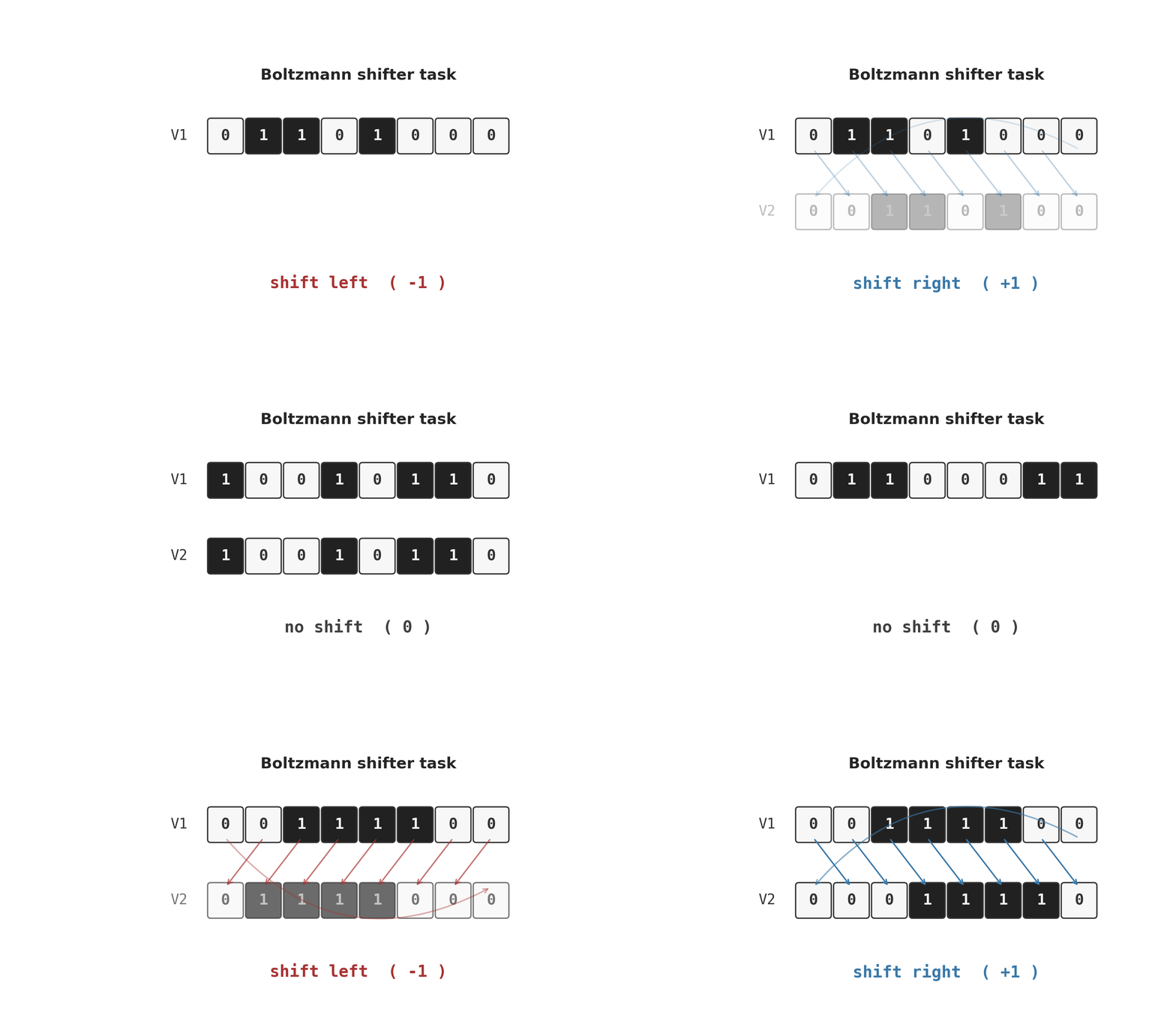
shifter — shifter Hinton & Sejnowski (1986), Learning and relearning in Boltzmann machines The canonical higher-order-feature toy: a Boltzmann machine learning to decide whether two binary input strips are shifted left, right, or not at all.

grapheme-sememe — grapheme-sememe Hinton & Sejnowski (1986), Learning and relearning in Boltzmann machines A 4-stage protocol, train, lesion, partial relearning, test, measuring spontaneous recovery: the network re-acquires lesioned associations faster than fresh ones, even without explicit retraining on them.

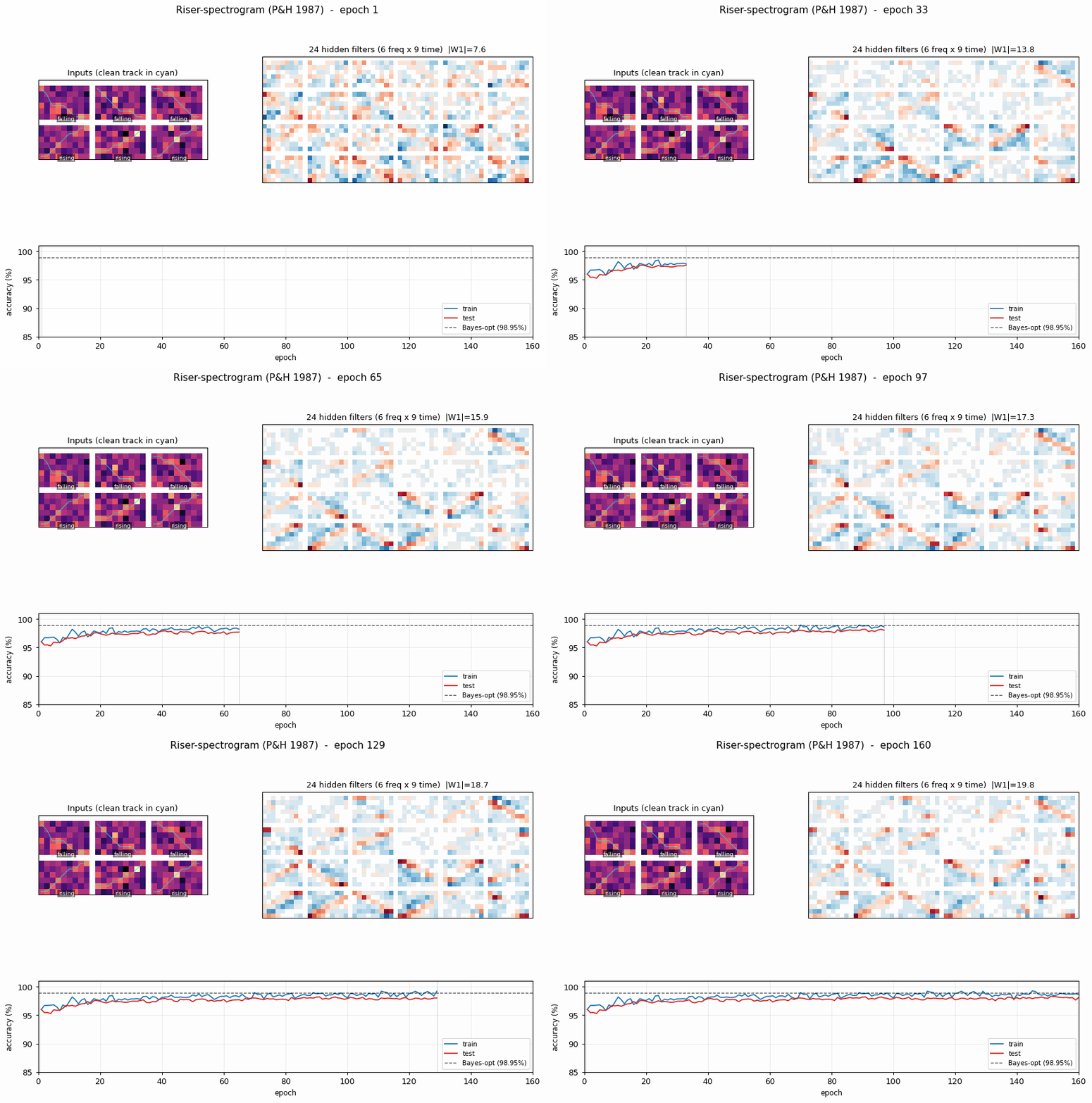
riser-spectrogram — riser-spectrogram Plaut & Hinton (1987), Learning sets of filters using back-propagation Synthetic riser/non-riser spectrogram discrimination. The interesting number is the gap to the analytically-known Bayes optimum: paper reports +1.0pp, we get +0.83pp, a small, real gap that goes away with longer training.

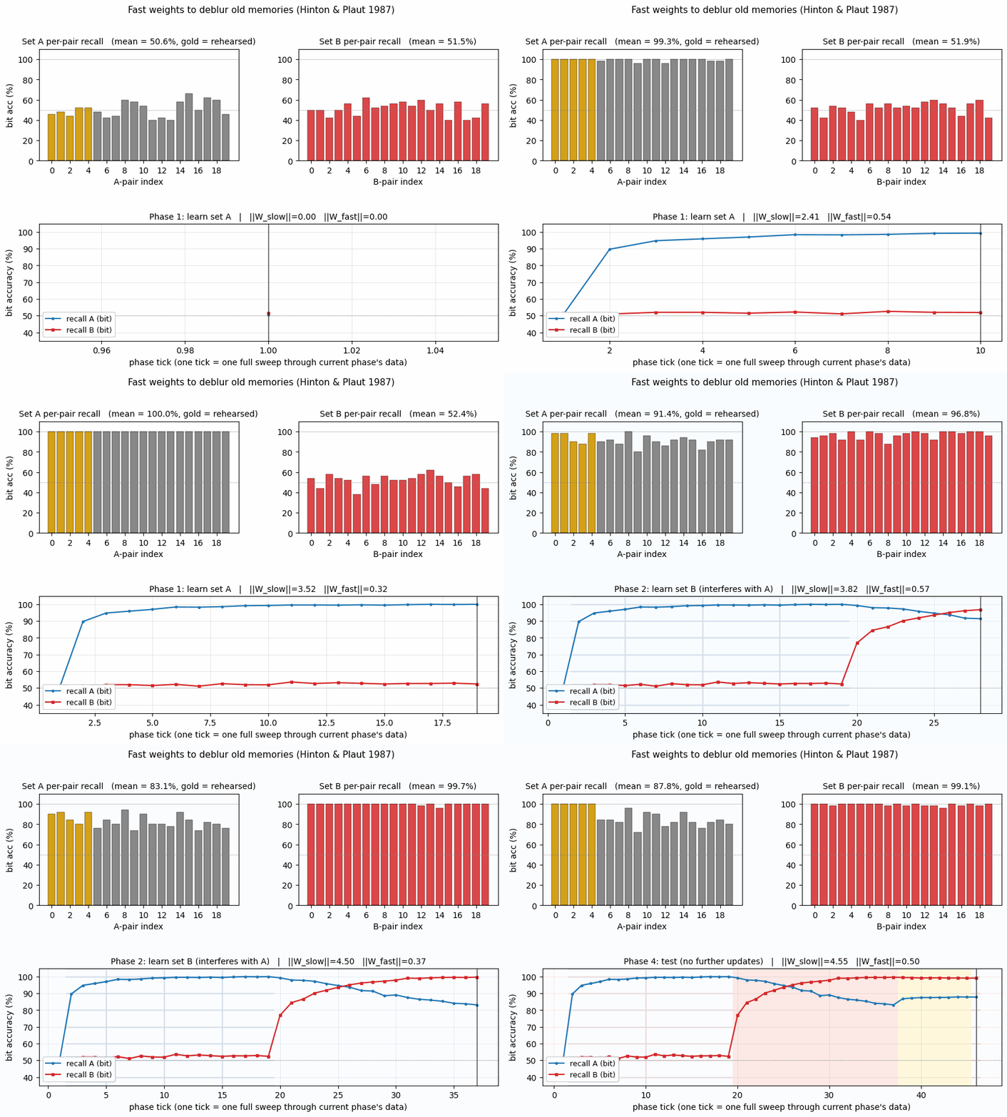
fast-weights-rehearsal — fast-weights-rehearsal Hinton & Plaut (1987), Using fast weights to deblur old memories Two-time-scale weights, slow weights store the long-term memory; fast weights pull old memories back into focus when rehearsal stimuli appear. The GIF runs the 4-phase protocol;

1990s, Unsupervised learning, mixtures, the Helmholtz machine

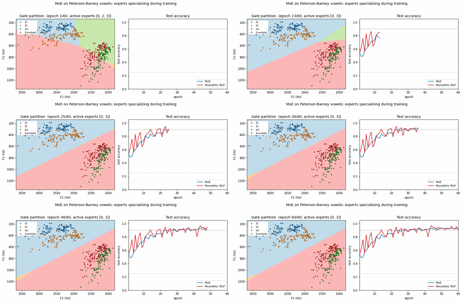
vowel-mixture-experts — vowel-mixture-experts Jacobs, Jordan, Nowlan & Hinton (1991), Adaptive mixtures of local experts Peterson-Barney 4-class vowels in F1/F2 space. The gate's softmax over experts ends up cleanly partitioning the vowel space along phonetic boundaries, exactly the "competing experts" picture the paper sells. 2.7pp gain over a parameter-matched MLP.

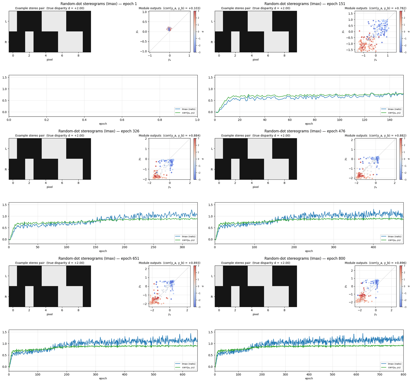
random-dot-stereograms — random-dot-stereograms Becker & Hinton (1992), A self-organizing neural network that discovers surfaces in random-dot stereograms Imax / spatial-coherence objective on synthetic random-dot stereograms. The model discovers depth (disparity) without any depth supervision, pure mutual-information between adjacent receptive fields. Disparity readout R² = 0.74 with no labels.

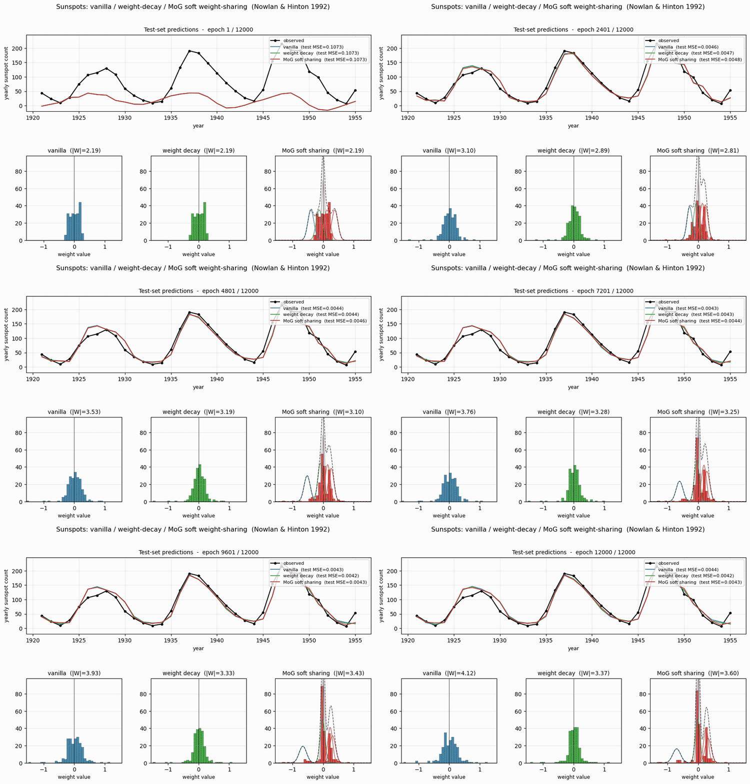
sunspots — sunspots Nowlan & Hinton (1992), Simplifying neural networks by soft weight-sharing Soft weight-sharing on Wolfer sunspot-count regression. The post-training weight histogram develops two clean Gaussian peaks (one at 0, pruned weights, and one at 0.27, shared non-zero value), exactly as the paper predicts.

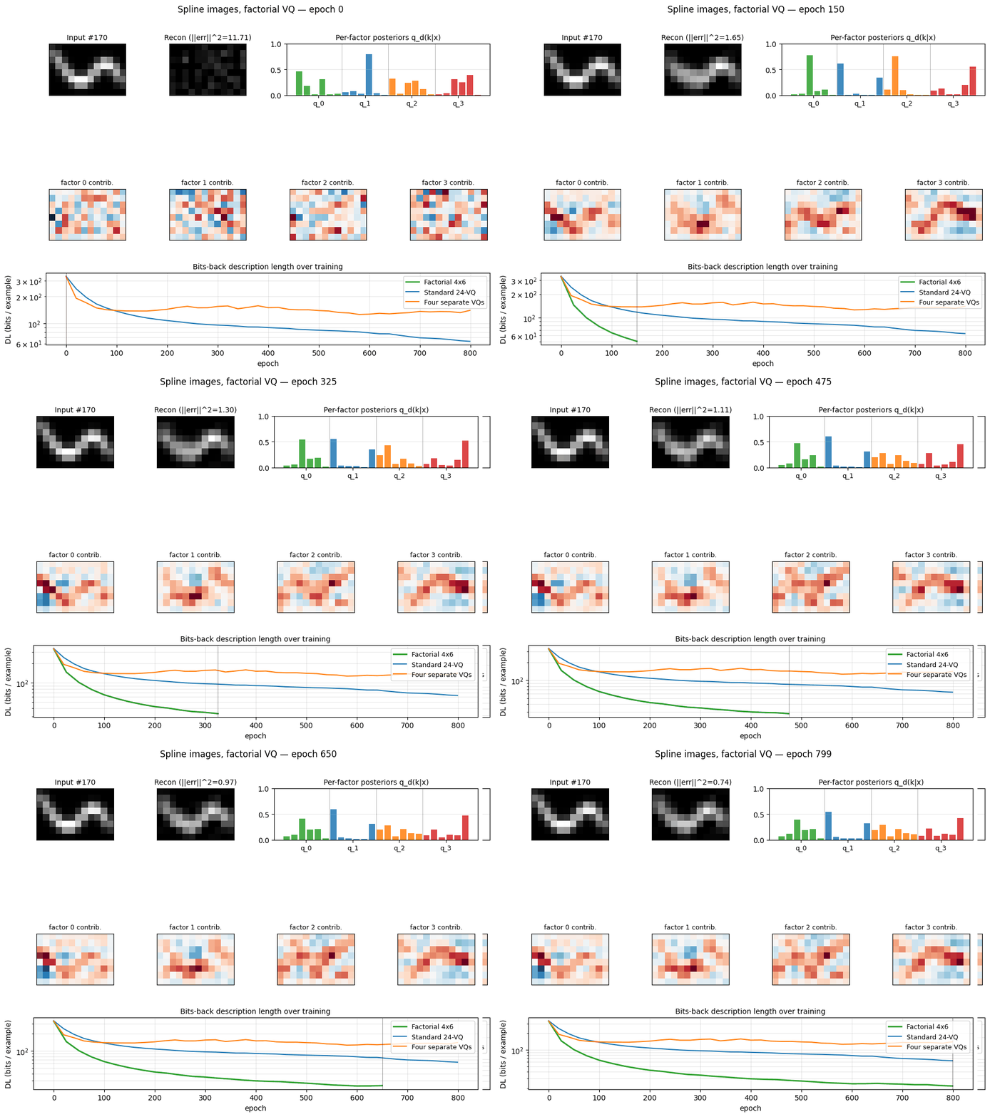
spline-images-factorial-vq — ★ spline-images-factorial-vq Hinton & Zemel (1994), Autoencoders, MDL and Helmholtz free energy Synthetic 5-parameter spline curves rendered to 2D images. The MDL factorial VQ assigns one VQ per latent dimension and beats a single 24-codebook standard-VQ baseline 3×.

dipole-position — dipole-position Zemel & Hinton (1995), Learning population codes by minimizing description length 8×8 dipole at random (x, y). Population code emerges as a 2D arrangement of receptive fields tiling the input plane. Needs a brief supervised warm-up to break the symmetry, once broken, R² = 0.81.

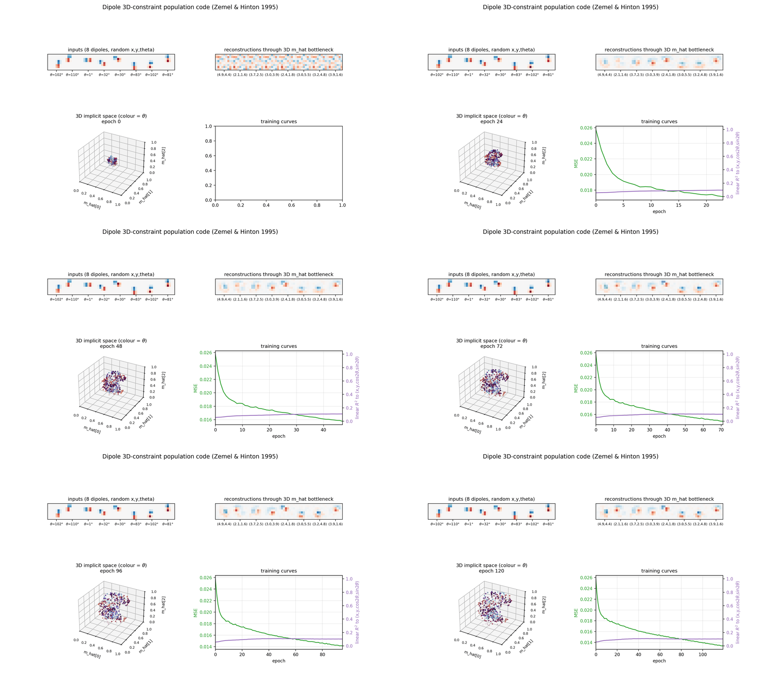
dipole-3d-constraint — dipole-3d-constraint Zemel & Hinton (1995), Learning population codes by minimizing description length The 2D positions are constrained to lie on a 3D constraint surface; the network discovers all three dimensions of the manifold.

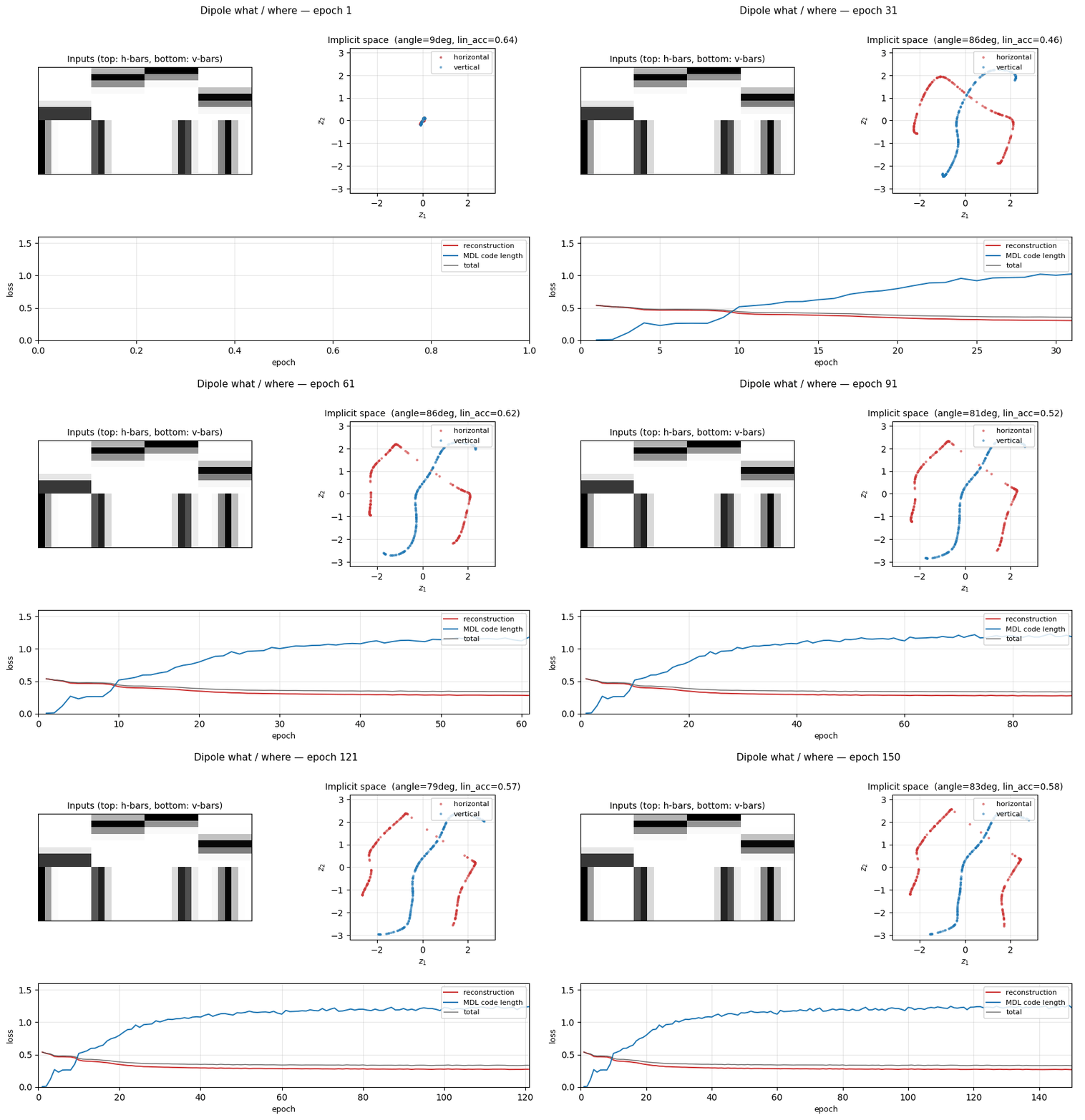
dipole-what-where — dipole-what-where Zemel & Hinton (1995), Learning population codes by minimizing description length Discontinuous what/where bars, the latent space splits into two perpendicular manifolds (identity vs location). Linear separability 0.58 shows the split, not perfectly clean.

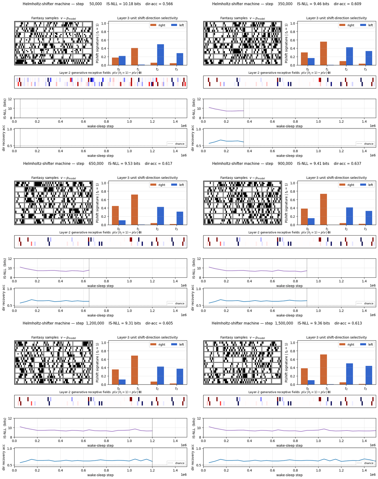
helmholtz-shifter — helmholtz-shifter Dayan, Hinton, Neal & Zemel (1995), The Helmholtz machine Two-stage generative shifter, recognition net + generative net trained by wake-sleep. 3 of 4 top-layer units become shift-selective; the generative model produces visually plausible shifted samples in the sleep phase shown in the GIF.

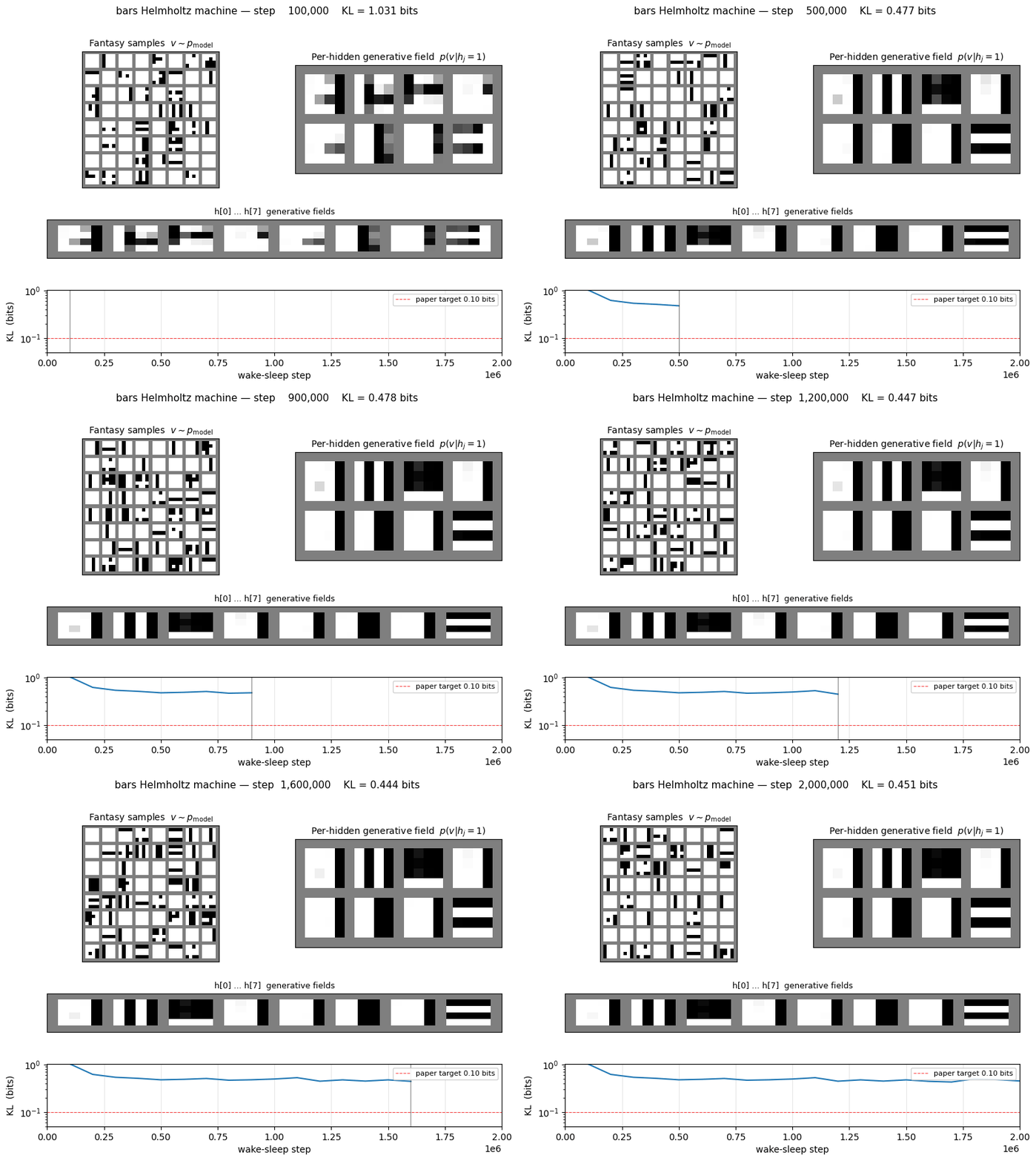
bars — bars Hinton, Dayan, Frey & Neal (1995), The wake-sleep algorithm The 4×4 horizontal/vertical bars problem, one of the most-cited toy generative-modelling benchmarks. 16-8-1 sigmoid belief net trained by wake-sleep. The KL gap to the paper number (0.451 vs 0.10) is documented as a partial reproduction;

2000s, Products of experts and temporal RBMs

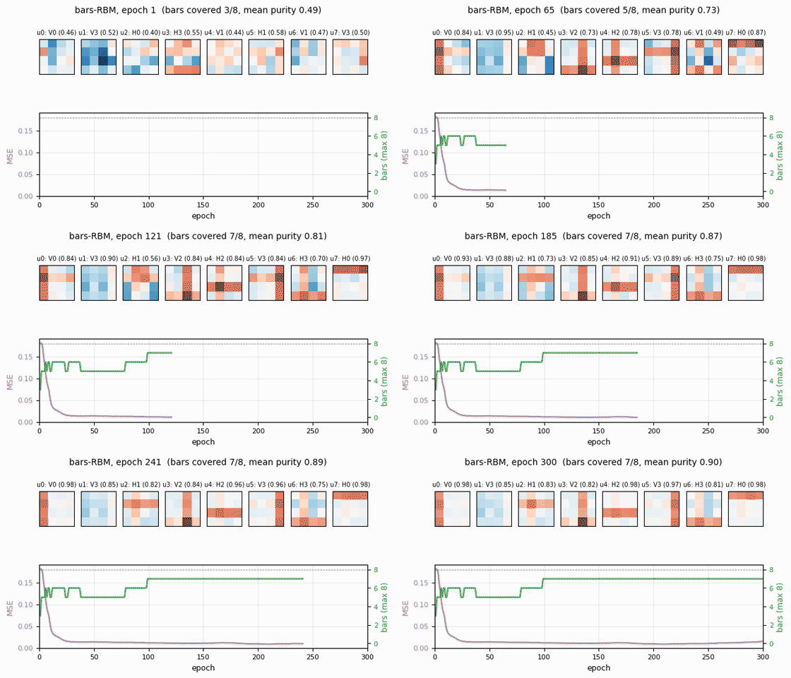
bars-rbm — bars-rbm Hinton (2000), Training products of experts by minimizing contrastive divergence The same bars problem trained as a CD-k RBM rather than wake-sleep. With 8 hidden units 7 of 8 bars are recovered cleanly; bumping to 16 hidden units recovers all 8. Direct demonstration of why CD made unsupervised learning at scale tractable.

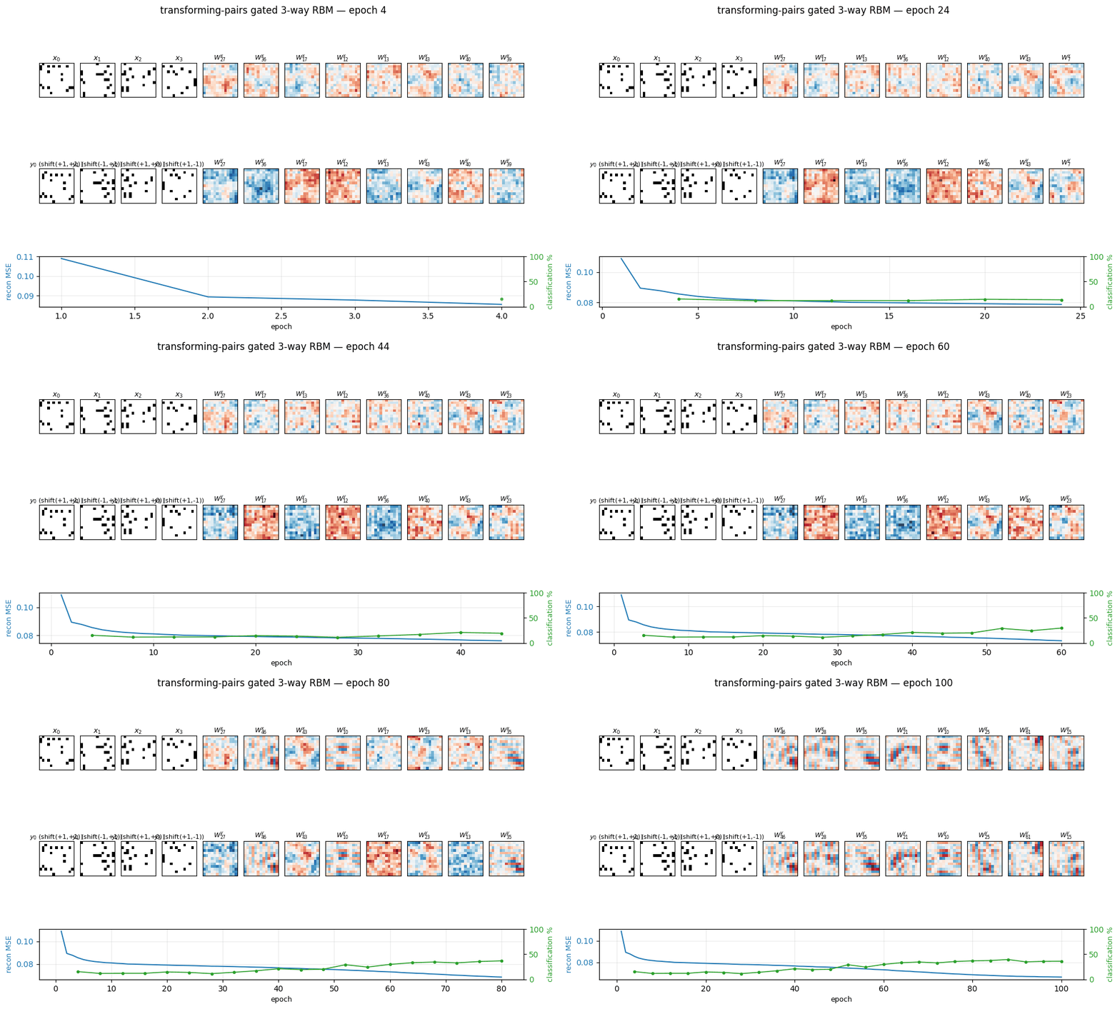
transforming-pairs — transforming-pairs Memisevic & Hinton (2007), Unsupervised learning of image transformations Gated 3-way RBM, the gates encode the transformation between two images, not either image alone.

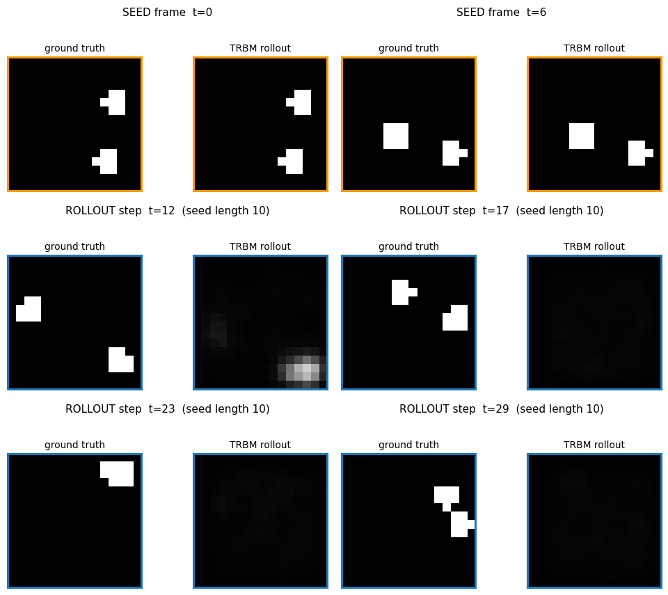
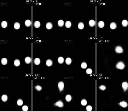
bouncing-balls-2 — bouncing-balls-2 Sutskever & Hinton (2007), Multilevel distributed representations for high-dimensional sequences TRBM video of bouncing balls. Rollout MSE sits between the trivial "copy last frame" and the oracle baselines, model has clearly learned some dynamics but not perfect physics.

bouncing-balls-3 — bouncing-balls-3 Sutskever, Hinton & Taylor (2008), The recurrent temporal RBM Same domain at higher resolution (30×30) and the recurrent variant. Reconstruction is tight (0.005 MSE on next-frame given history); free rollout drifts to 0.13, the classic accumulating-error story.

2010s, Capsules, distillation, attention

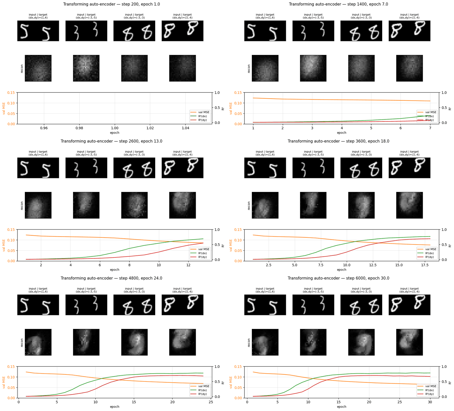
transforming-autoencoders — transforming-autoencoders Hinton, Krizhevsky & Wang (2011), Transforming auto-encoders The seed of the capsules program. Each capsule outputs a small pose vector (dx, dy) per part; reconstruction is gated through that pose.

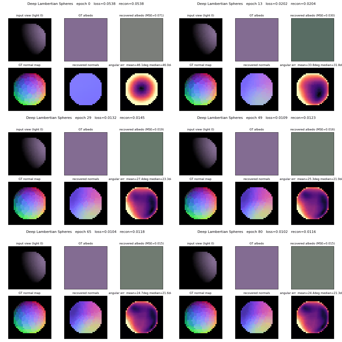
deep-lambertian-spheres — deep-lambertian-spheres Tang, Salakhutdinov & Hinton (2012), Deep Lambertian Networks Synthetic spheres rendered under multiple lighting directions. The model recovers surface normals (27° angular error) and albedo (7× better than naive baseline) by separating shading from reflectance, the intrinsic-images problem cast as inverse.

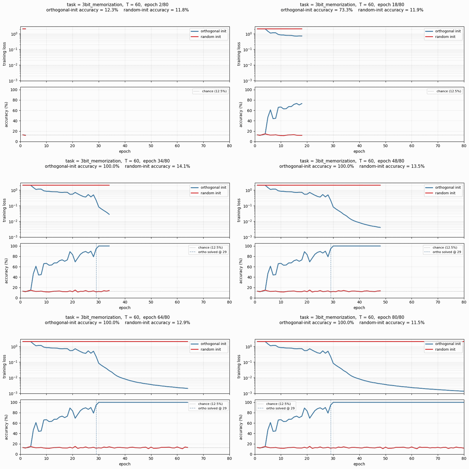
rnn-pathological — rnn-pathological Sutskever, Martens, Dahl & Hinton (2013), On the importance of initialization and momentum The Hochreiter-Schmidhuber long-term-dependency battery. 3 of 4 tasks solved; orthogonal initialization beats random Gaussian init by a clear margin in the wallclock-to-converge curve.

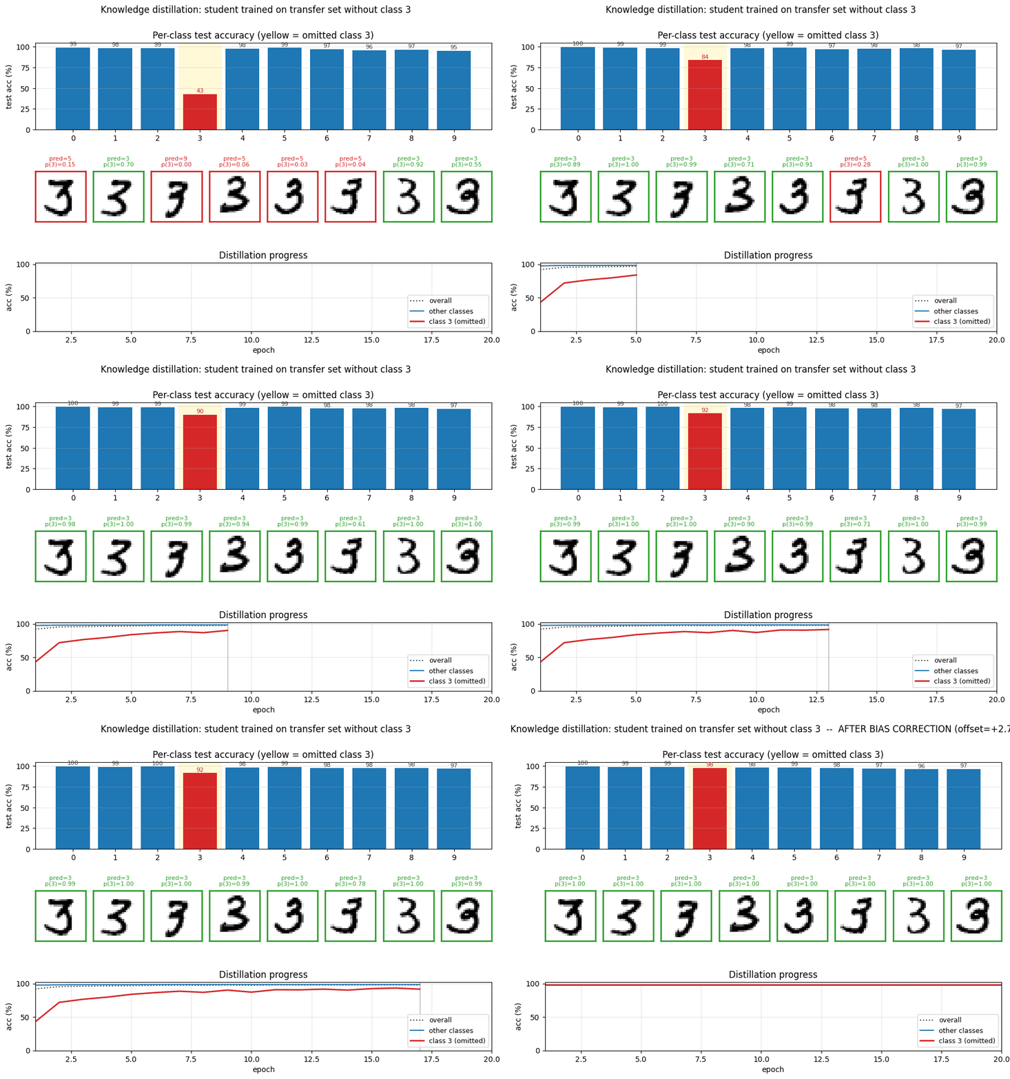
distillation-mnist-omitted-3 — distillation-mnist-omitted-3 Hinton, Vinyals & Dean (2015), Distilling the knowledge in a neural network The classic "student never sees a 3" demonstration. Soft-target distillation transfers enough information about digit 3 from the teacher's logits that, after a per-class bias correction, the student classifies 3s at 97.82%.

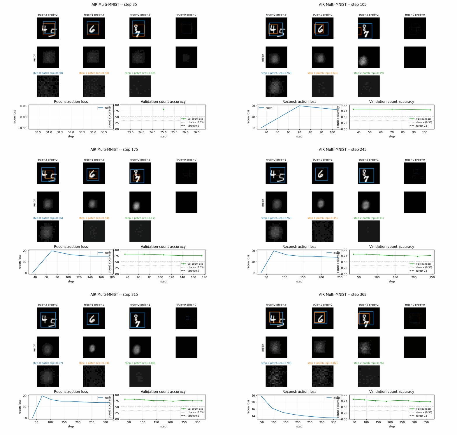
air-multimnist — air-multimnist Eslami et al. (2016), Attend, Infer, Repeat Variable-count MNIST scenes, the model decides how many objects are in the image, then attends to and reconstructs each. Object-count accuracy 79.7%; reconstructions blurry. The GIF visualizes the per-step attention windows opening one at a time.

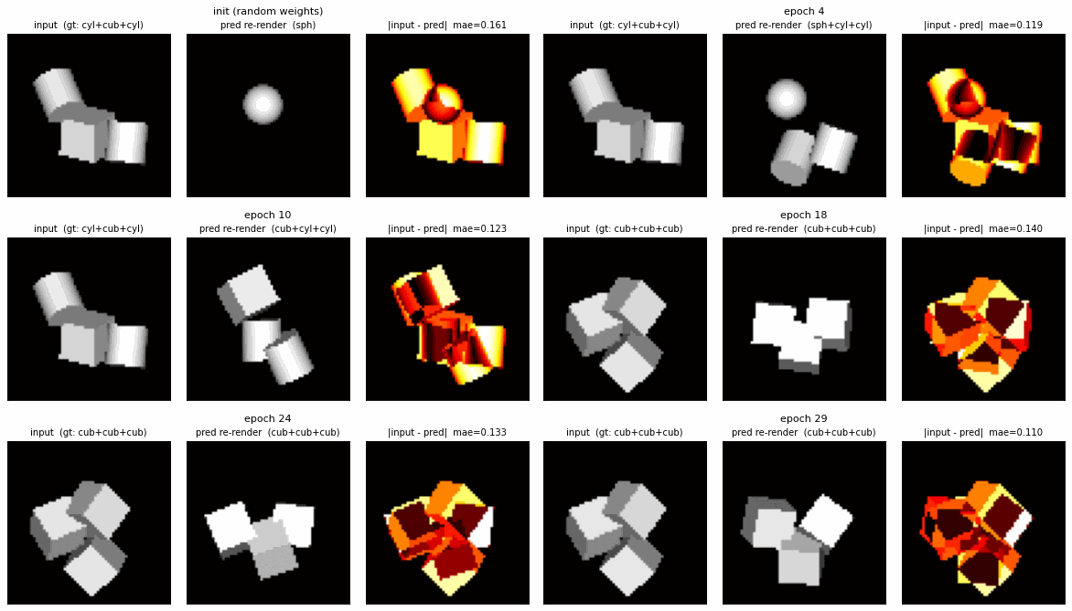
air-3d-primitives — air-3d-primitives Eslami et al. (2016), Attend, Infer, Repeat Same AIR machinery, but the renderer is a small 3D primitive engine and the inference network must invert it. Cleanly recovers 1-primitive scenes; 3-primitive count accuracy 81%.

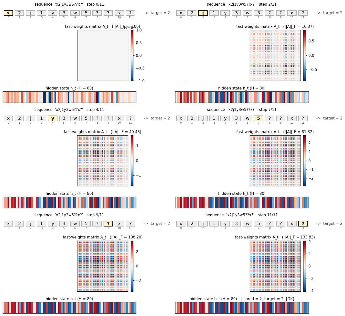
fast-weights-associative-retrieval — fast-weights-associative-retrieval Ba, Hinton, Mnih, Leibo & Ionescu (2016), Using fast weights to attend to the recent past faithful; retrieval rate 38% short of paper. The fast-weight matrix (visualized as a heatmap that grows then decays) is the visualization star here.

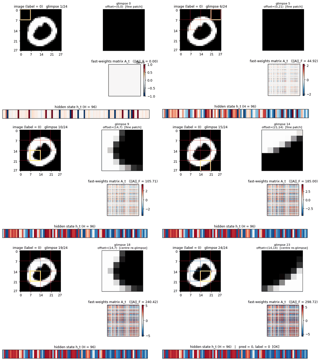
multi-level-glimpse-mnist — multi-level-glimpse-mnist Ba, Hinton, Mnih, Leibo & Ionescu (2016), Using fast weights to attend to the recent past 24 hierarchical glimpses on MNIST. The GIF traces the glimpse trajectory across the digit, a clean visualization of attention-as-control even at the modest 82% accuracy.

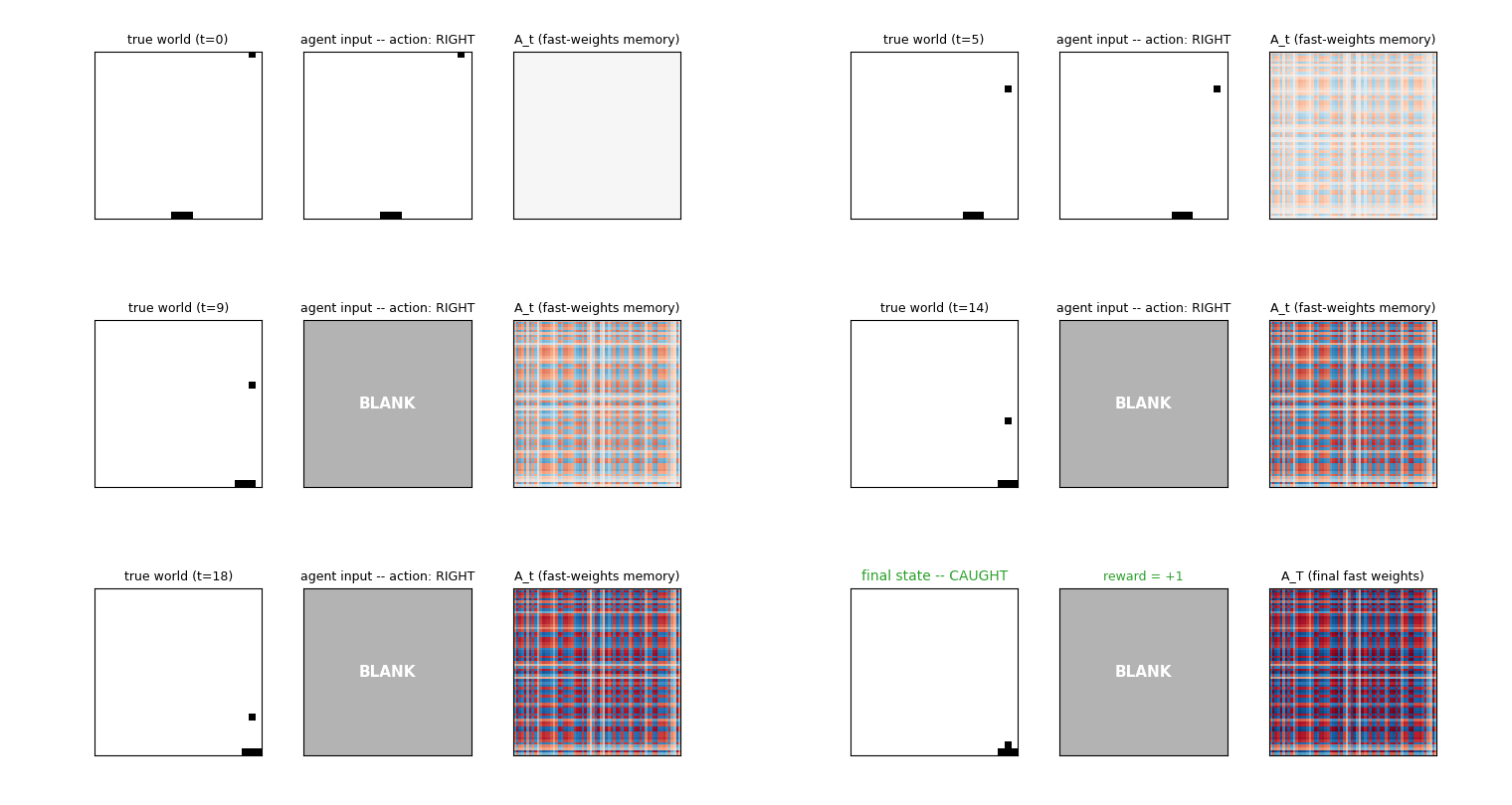
catch-game — catch-game Ba, Hinton, Mnih, Leibo & Ionescu (2016), Using fast weights to attend to the recent past A partial-observability paddle/ball game where the network must integrate information across time to catch the ball. Fast-weights variant beats the vanilla RNN 33.9% to 11.4% at size=20 (paper-scale); reaches 91% at the easier size=10 setting.

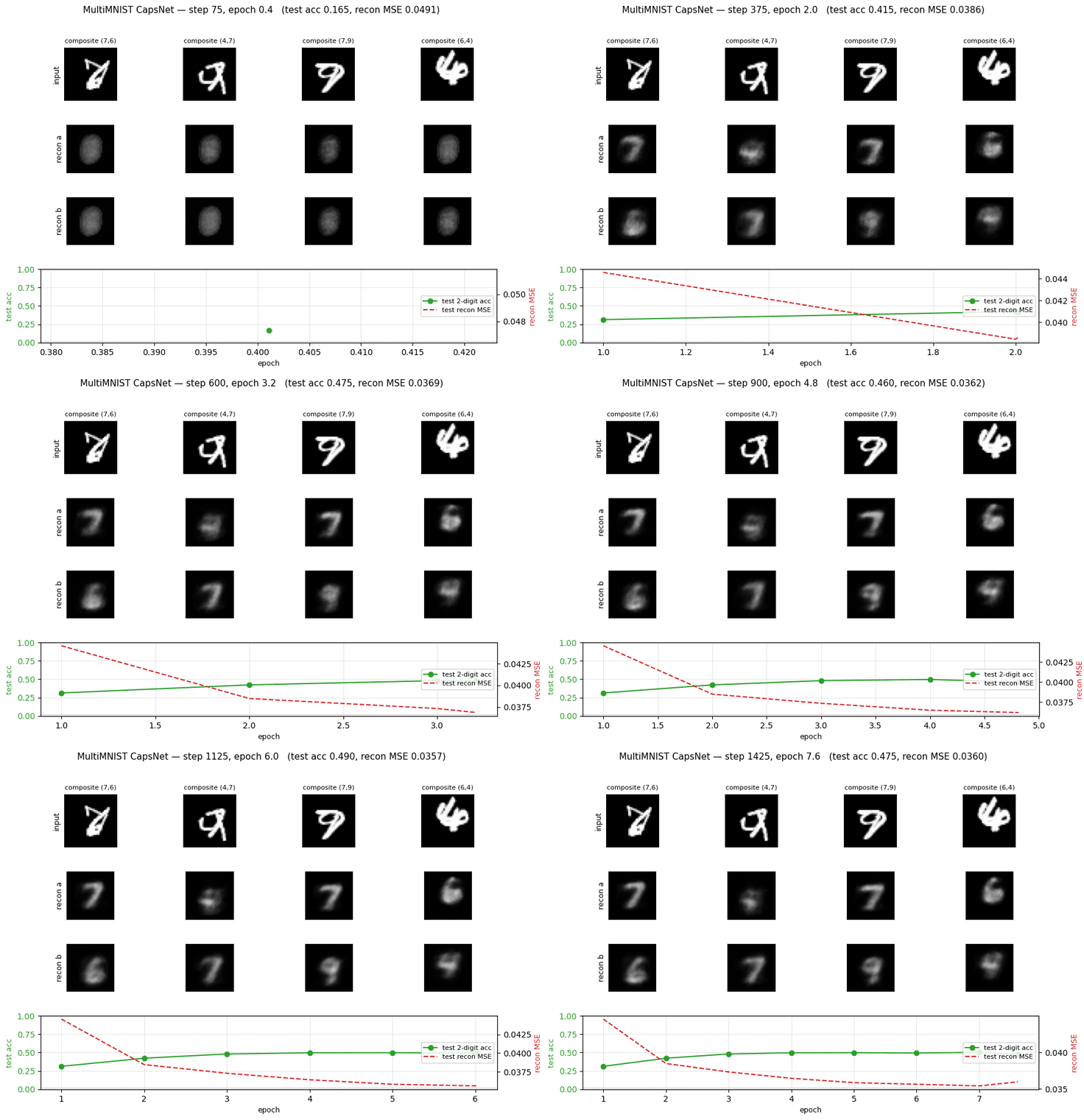
multimnist-capsnet — multimnist-capsnet Sabour, Frosst & Hinton (2017), Dynamic routing between capsules Overlapping digit pairs. The network must decompose a single image into two simultaneous classifications, exactly the case capsules were designed for. 22× above chance at 48.6% on this hard split, but well short of paper.

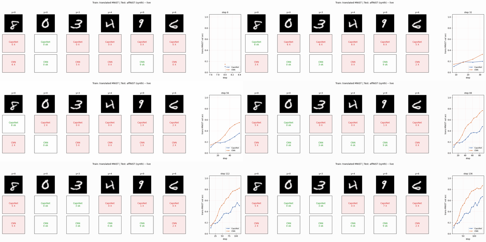
affnist — affnist Sabour, Frosst & Hinton (2017), Dynamic routing between capsules Train on translated MNIST, test on affNIST (additional rotations and shears). The paper claimed CapsNet generalizes to novel viewpoints better than a parameter-matched CNN by +13%; we get the opposite sign.

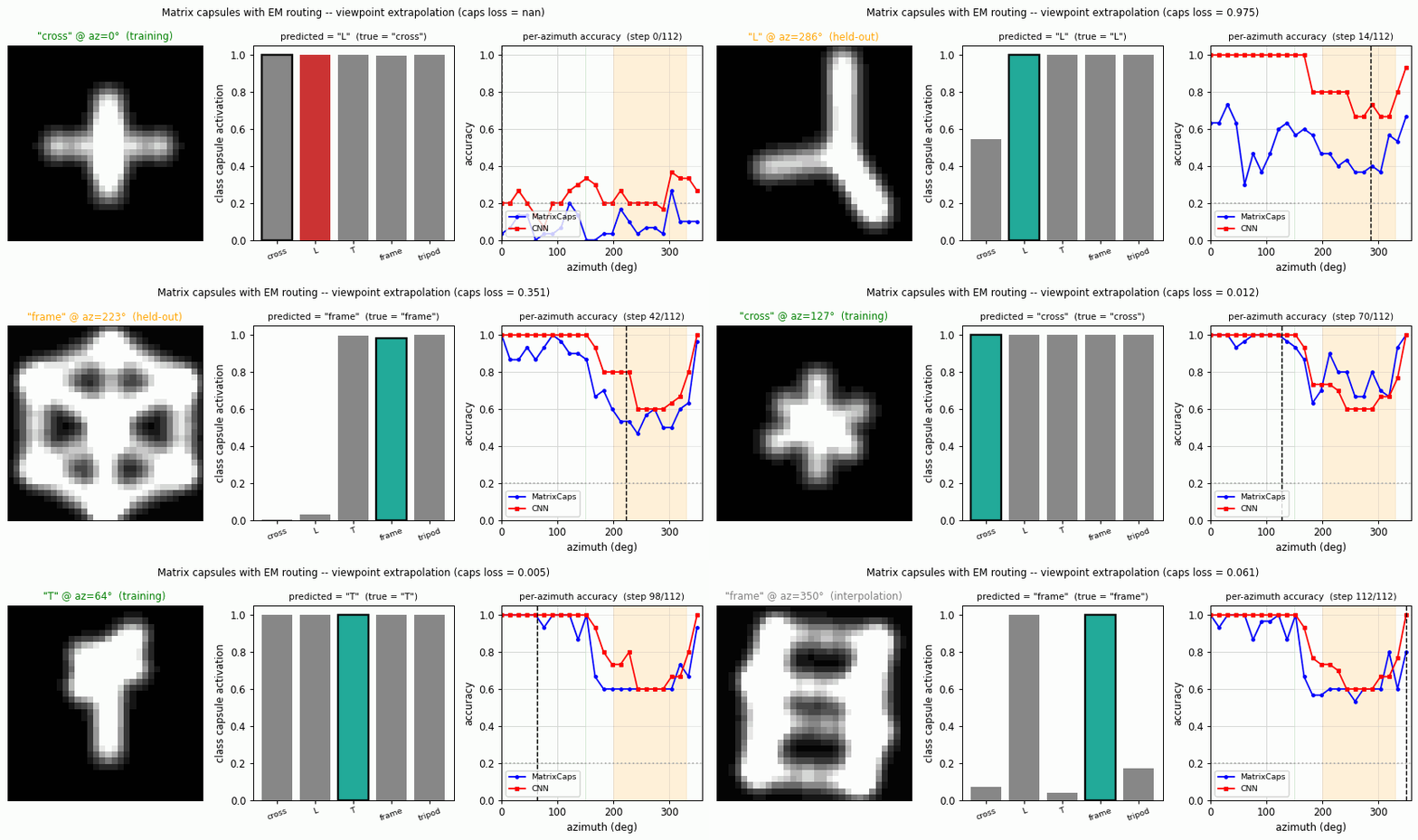
smallnorb-novel-viewpoint — smallnorb-novel-viewpoint Hinton, Sabour & Frosst (2018), Matrix capsules with EM routing Synthesized NORB-style objects, held-out azimuth/elevation at test time. Matrix capsules edge out a parameter-matched CNN on the held-out viewpoint split, the qualitative claim of the paper holds, with smaller absolute numbers.

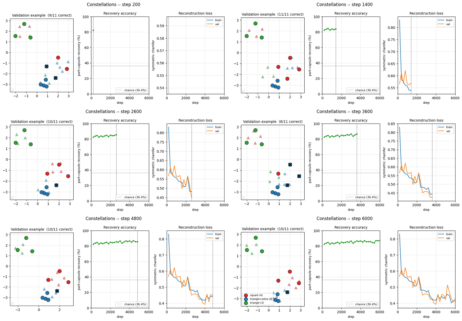
constellations — constellations Kosiorek, Sabour, Teh & Hinton (2019), Stacked capsule autoencoders 2D point-cloud part-whole grouping. The model groups individual points into the constellations they came from with no supervision, 86.9% per- point recovery at the best seed.

2020s, Subclass distillation, GLOM, Forward-Forward

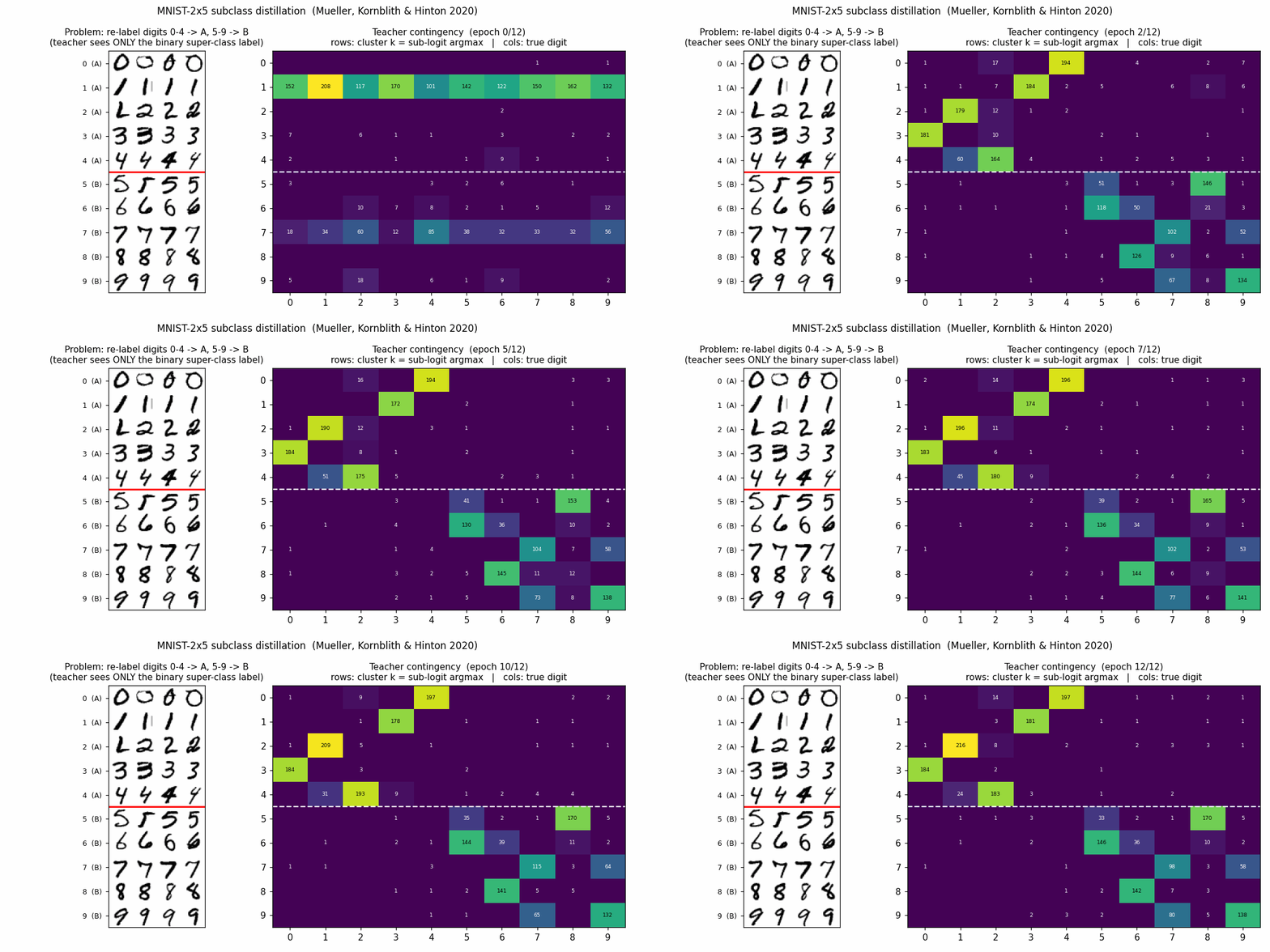
mnist-2x5-subclass — mnist-2x5-subclass Müller, Kornblith & Hinton (2020), Subclass distillation A super-class teacher trained on {0..4} vs {5..9} two-class labels; the student receives the teacher's logits, which carry hidden subclass information.

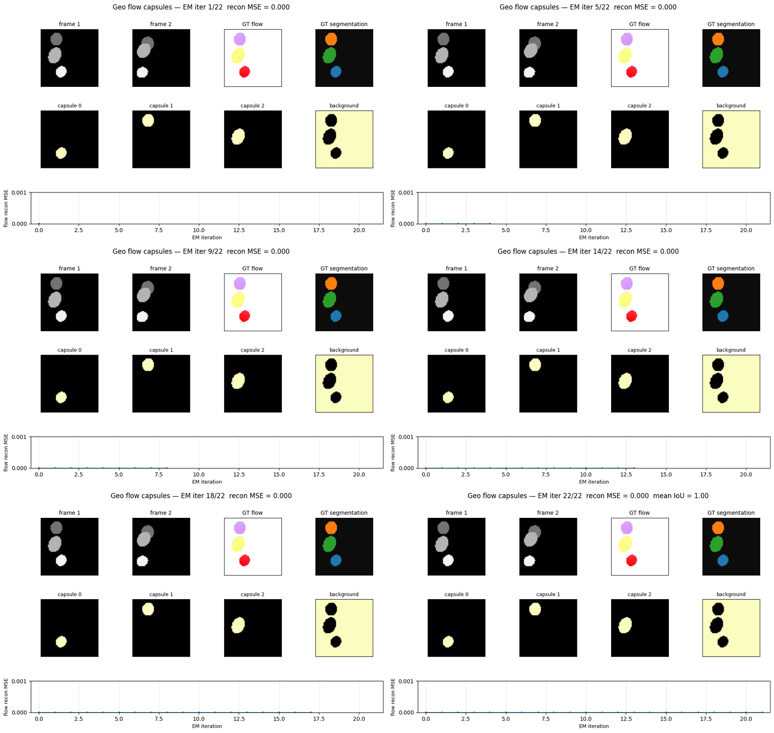
geo-flow-capsules — geo-flow-capsules Sabour, Tagliasacchi, Yazdani, Hinton & Fleet (2021), Unsupervised part representation by flow capsules Geo / Geo+ moving 2D shapes, the model decomposes each frame into parts using only motion (optical-flow consistency) as supervision. Mean IoU 0.764 against ground-truth part masks vs chance 0.20.

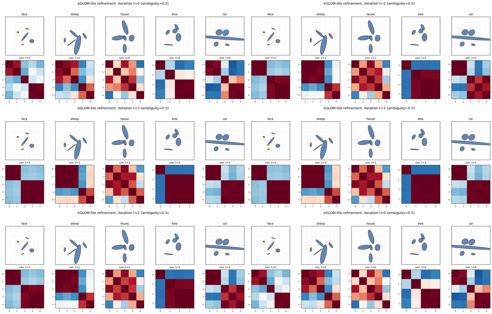
ellipse-world — ★ ellipse-world Culp, Sabour & Hinton (2022), Testing GLOM's ability to infer wholes from ambiguous parts eGLOM-lite for the ambiguous-part-to-whole test. Each frame of the GIF is one iteration of the GLOM column dynamics; you can watch islands of agreement form across iterations as ambiguous local parts commit to a consistent global whole.

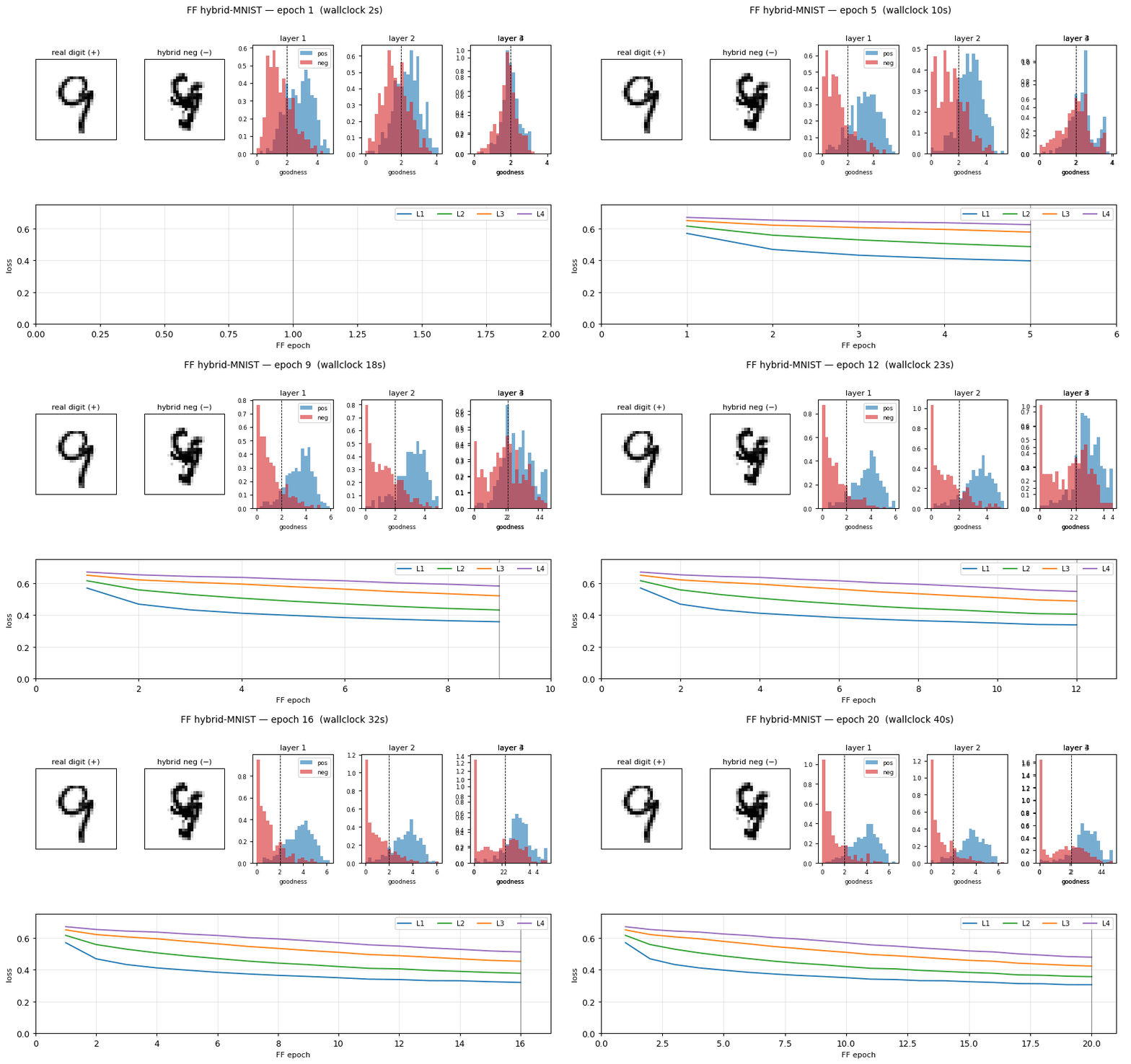
ff-hybrid-mnist — ff-hybrid-mnist Hinton (2022), The forward-forward algorithm FF unsupervised MLP with hand-crafted hybrid-image negatives. The GIF shows the negative-sample construction (images literally averaged in pixel space). Test error 5.21%, works, but does not match paper's 1.37%.

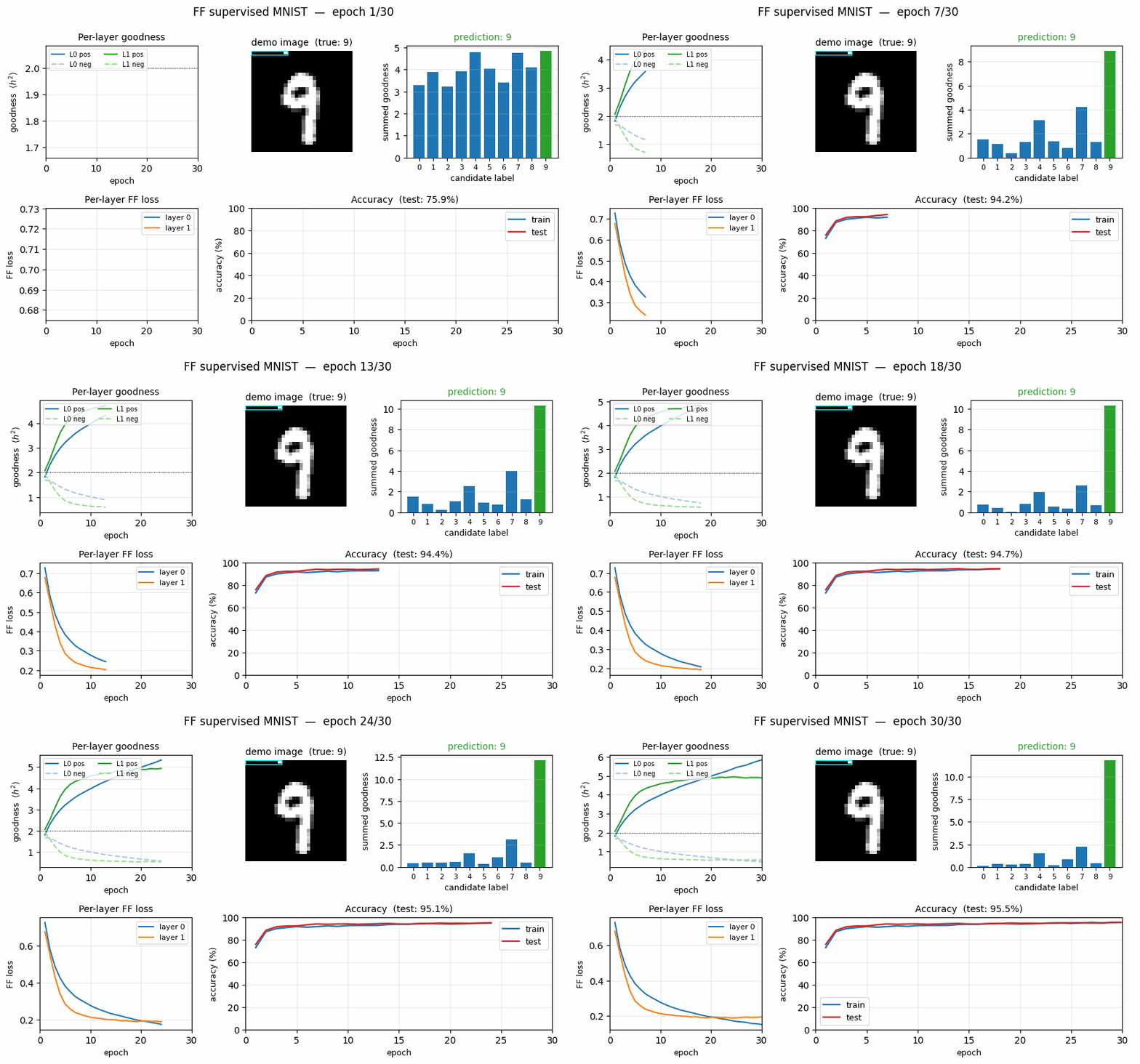
ff-label-in-input — ff-label-in-input Hinton (2022), The forward-forward algorithm The label one-hot is concatenated to the first 10 pixels of the image, then FF is run with the correct label as positive and a wrong label as negative. Closer to paper than the hybrid variant (3.60% vs 1.36%).

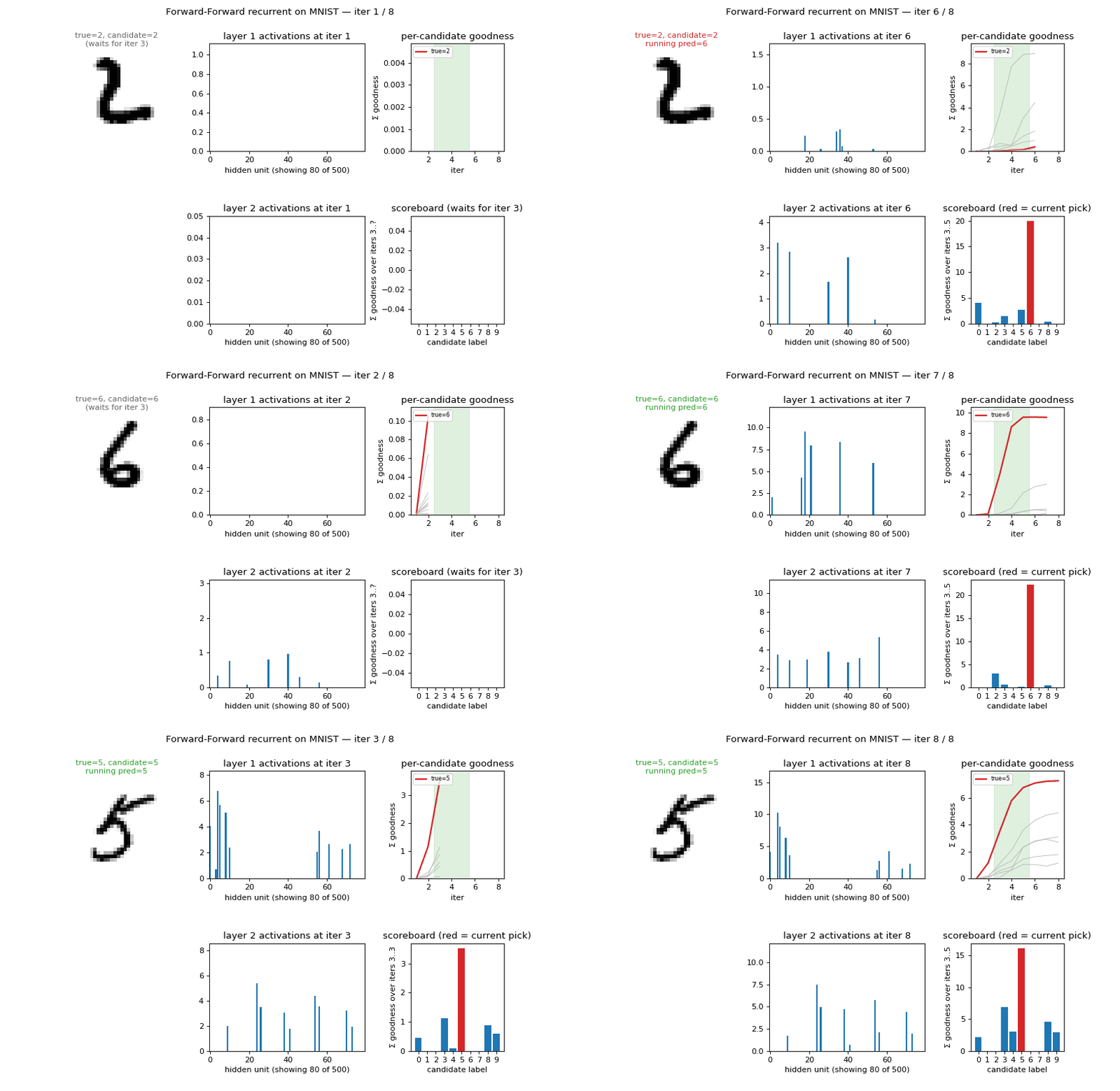
ff-recurrent-mnist — ★ ff-recurrent-mnist Hinton (2022), The forward-forward algorithm The "video" variant, the same MNIST frame repeated for several timesteps with top-down recurrent connections so each layer can use the next layer's previous-step activity as context.

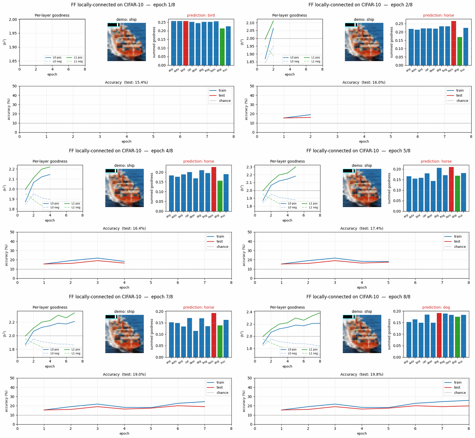
ff-cifar-locally-connected — ff-cifar-locally-connected Hinton (2022), The forward-forward algorithm CIFAR-10 with a locally-connected (not weight-tied) FF network. FF beats a parameter-matched BP baseline on this architecture (22.78% vs 38.31% test err), one of the few places in the suite where FF wins outright.

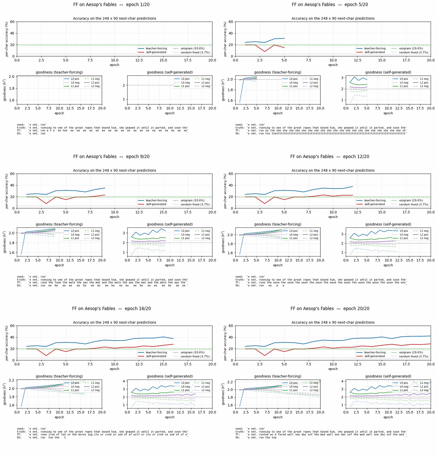
ff-aesop-sequences — ff-aesop-sequences Hinton (2022), The forward-forward algorithm Next-character prediction on Aesop's Fables with self-generated negatives, the negatives come from the model's own previous-step predictions. Teacher-forced 53%, self-generated 34%, well above any of the non-FF baselines (3-20%).

schmidhuber-problems 57 source tour

Jürgen Schmidhuber's catalog, 1989 onward, as runnable stubs.

1980s, Local rules and the Neural Bucket Brigade

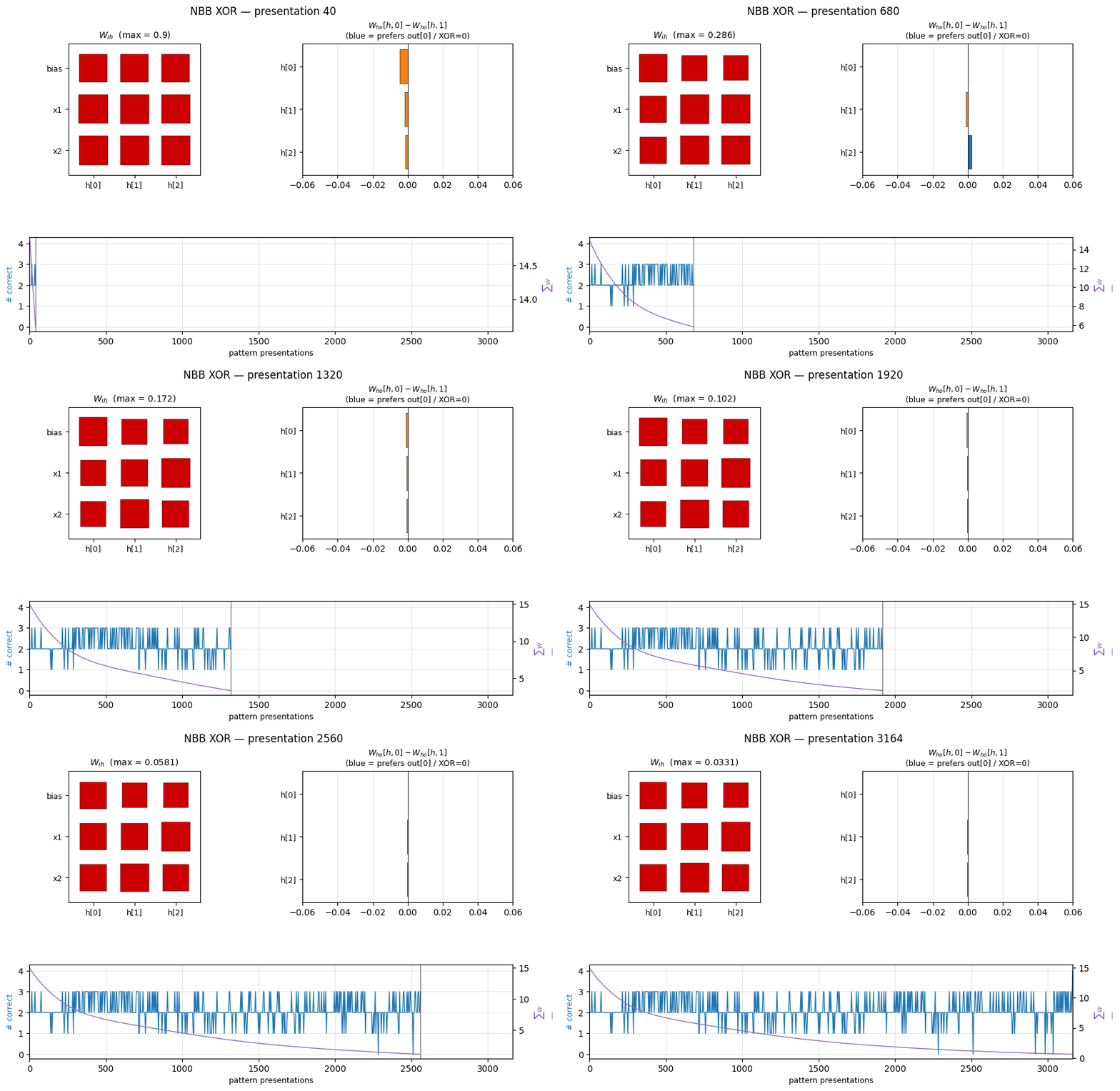
nbb-xor — nbb-xor Schmidhuber (1989), A local learning algorithm for dynamic feedforward and recurrent networks XOR via the Neural Bucket Brigade, a strictly local-in-space-and-time, winner-take-all, dissipative learning rule. There is no backprop, no RTRL, no gradient.

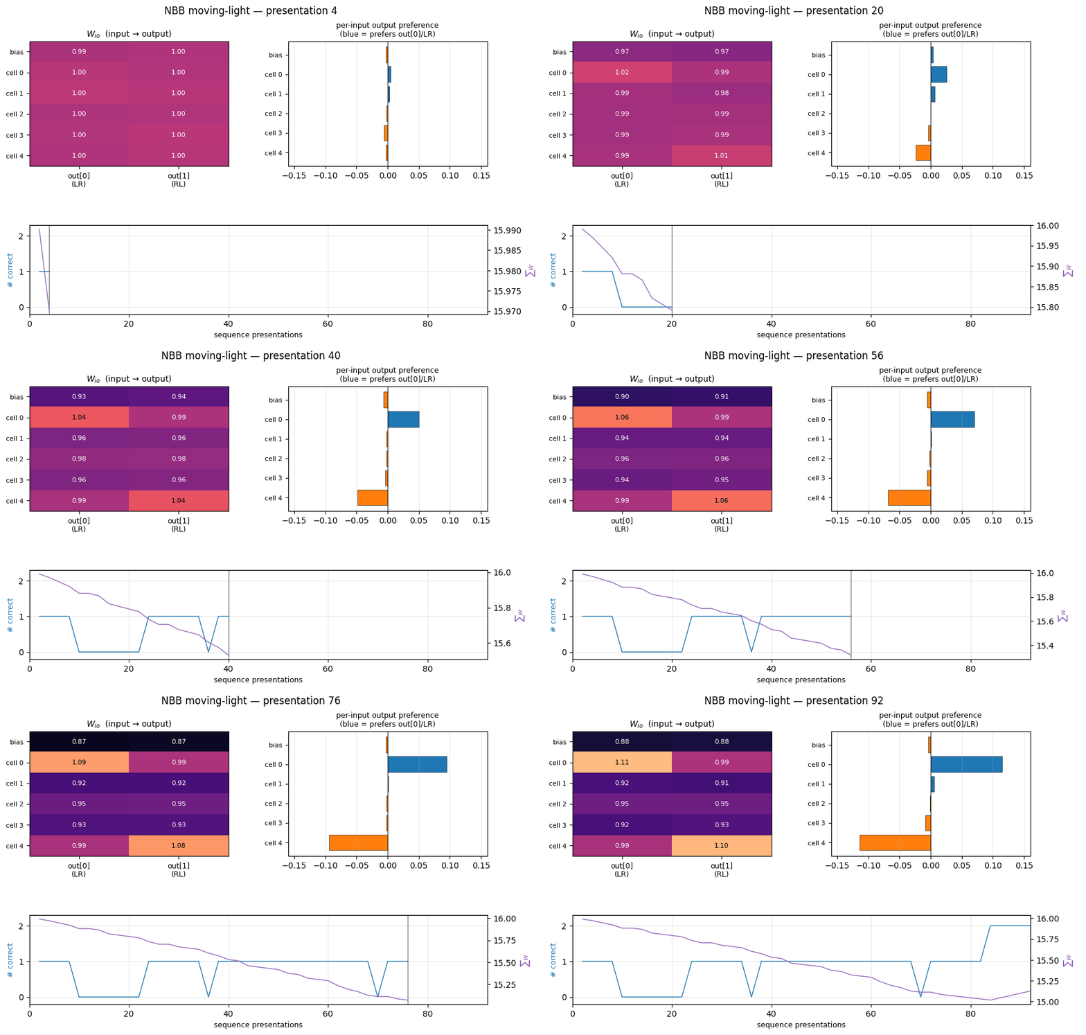
nbb-moving-light — nbb-moving-light Schmidhuber (1989), A local learning algorithm for dynamic feedforward and recurrent networks 1-D moving-light direction discrimination via the same NBB rule extended to a small fully-recurrent net (5 retina cells + bias to 2 output units forming a WTA subset).

1990, Controller + world-model + flip-flop

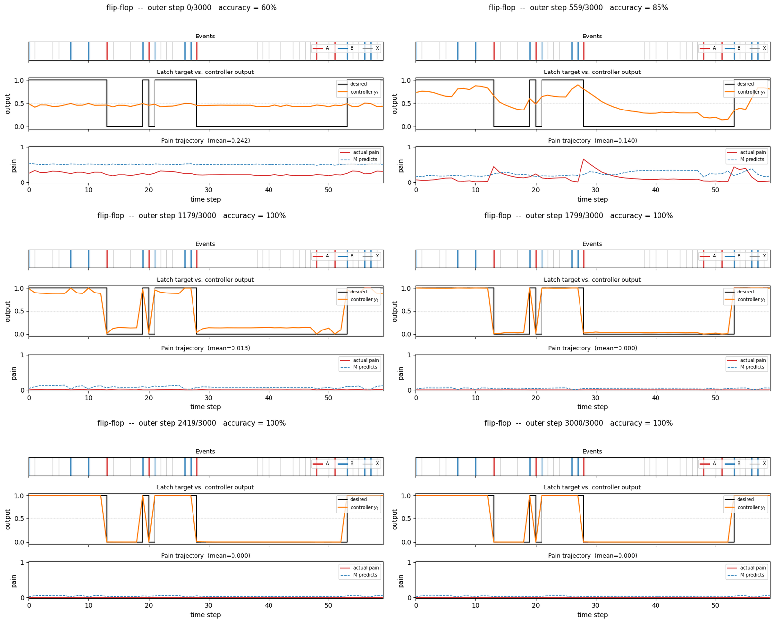
flip-flop — flip-flop Schmidhuber (1990), Making the world differentiable The 1990 paper sets up a tiny non-stationary control task that has all the ingredients of the long-time-lag problem Hochreiter would later formalise as the vanishing-gradient barrier.

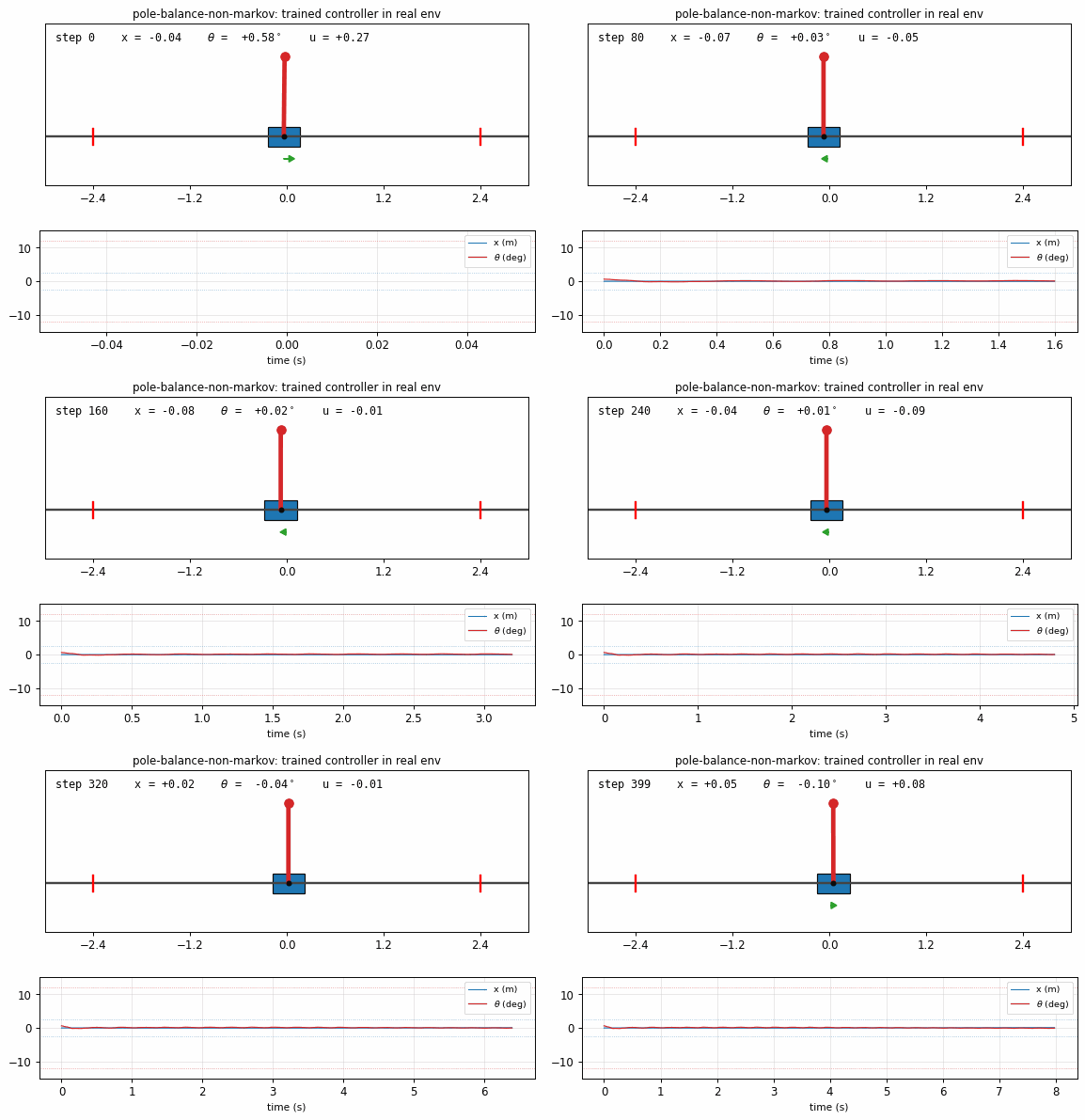
pole-balance-non-markov — pole-balance-non-markov Schmidhuber (1990), Making the world differentiable Cart-pole balancing where the controller observes only positions, not velocities. The 4-D real state is (x, x_dot, θ, θ_dot), but C only sees (x, θ). M predicts next observed positions from action + history; C trained by BP through M's gradient.

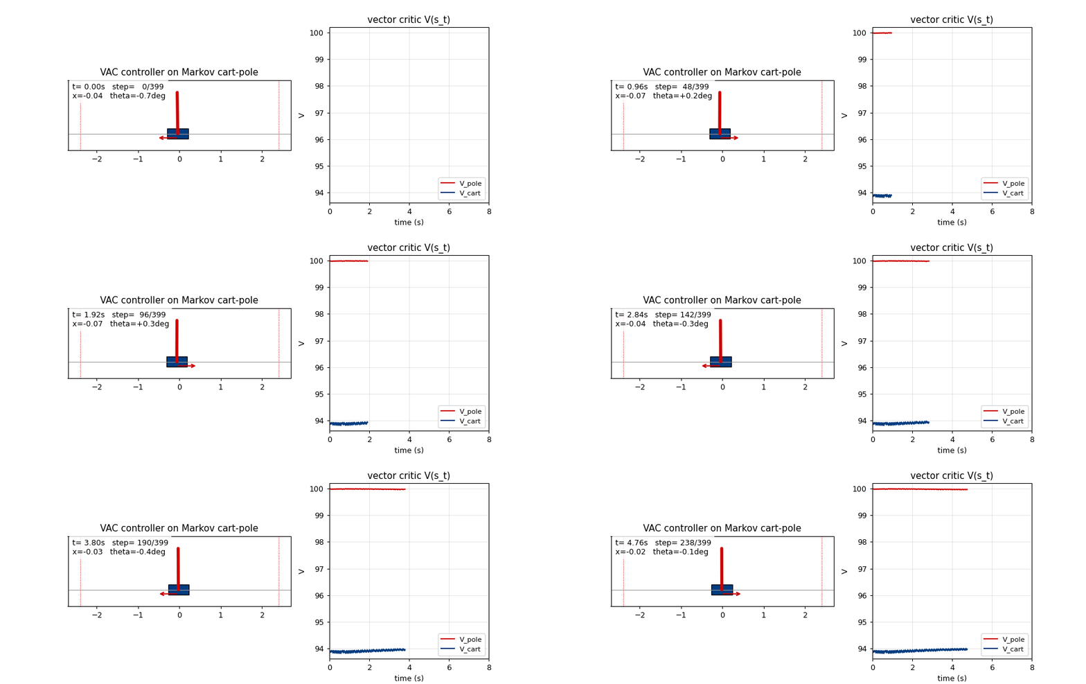
pole-balance-markov-vac — pole-balance-markov-vac Schmidhuber (1990), Recurrent networks adjusted by adaptive critics Standard cart-pole, Markov regime: the controller observes the full state at every step. K=2 vector-valued critic with two qualitatively distinct components (V_pole saturates near 1/(1-γ)=100; V_cart tracks live 1−|x|/2.4 margin).

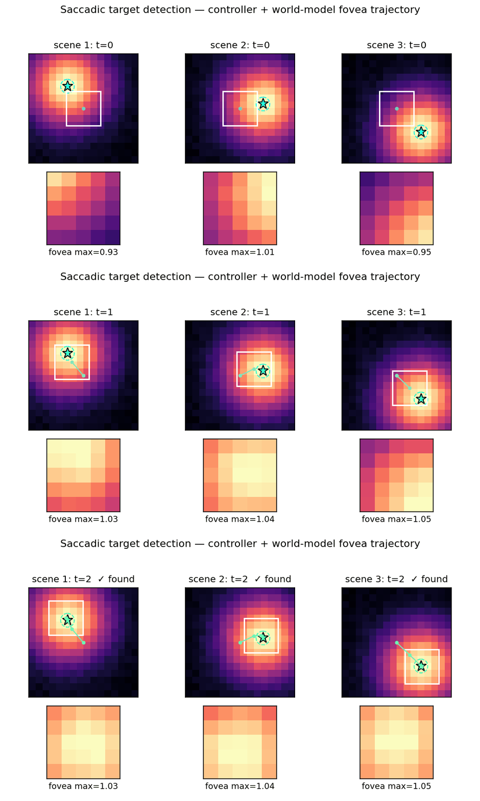
saccadic-target-detection — saccadic-target-detection Schmidhuber & Huber (1990), Learning to generate focus trajectories Active visual attention. The controller must move a small fovea over a 2-D scene to find a target halo, given only the local pixels under the fovea. C is feedforward; M predicts the change in halo at the next fovea position.

1991, Curiosity, subgoals, the chunker

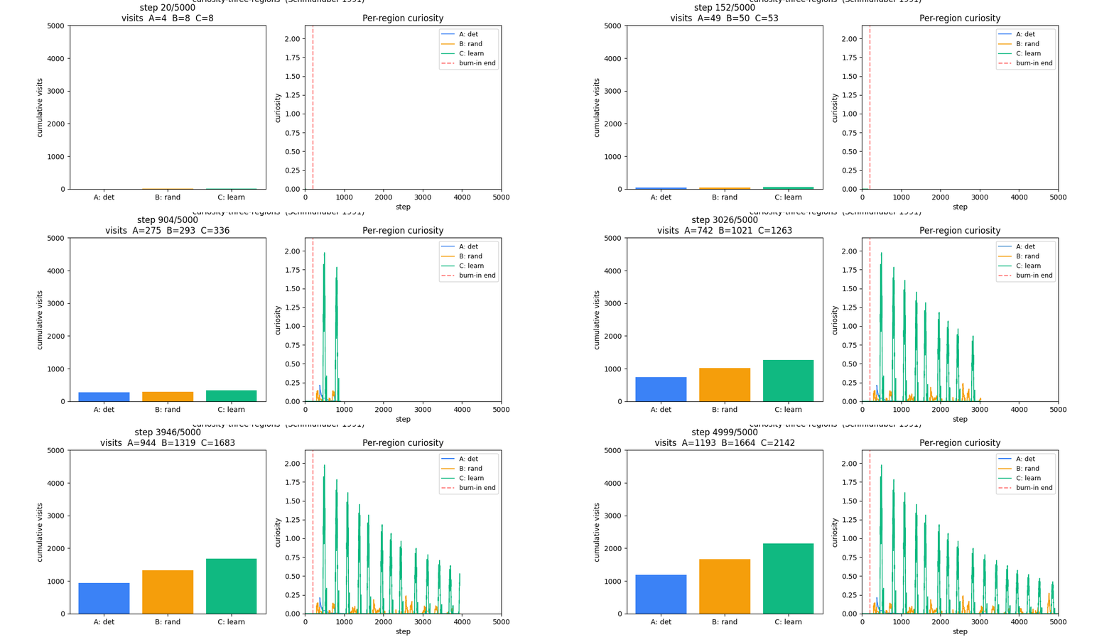
curiosity-three-regions — curiosity-three-regions Schmidhuber (1991), Adaptive confidence and adaptive curiosity A 1-D environment partitioned into three regions: deterministic / random / learnable-but-unlearned. Curiosity reward = windowed reduction in M's prediction error.

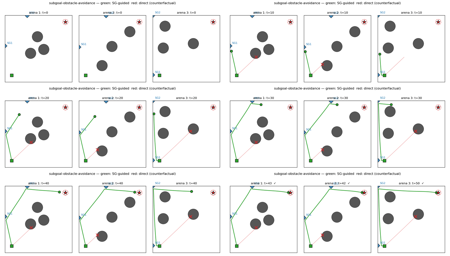
subgoal-obstacle-avoidance — subgoal-obstacle-avoidance Schmidhuber (1991), Learning to generate sub-goals for action sequences Hierarchical RL: a sub-goal generator C_high proposes K=2 waypoints, a low-level controller C_low (intentionally obstacle-blind, input = rel_target only) steers toward each.

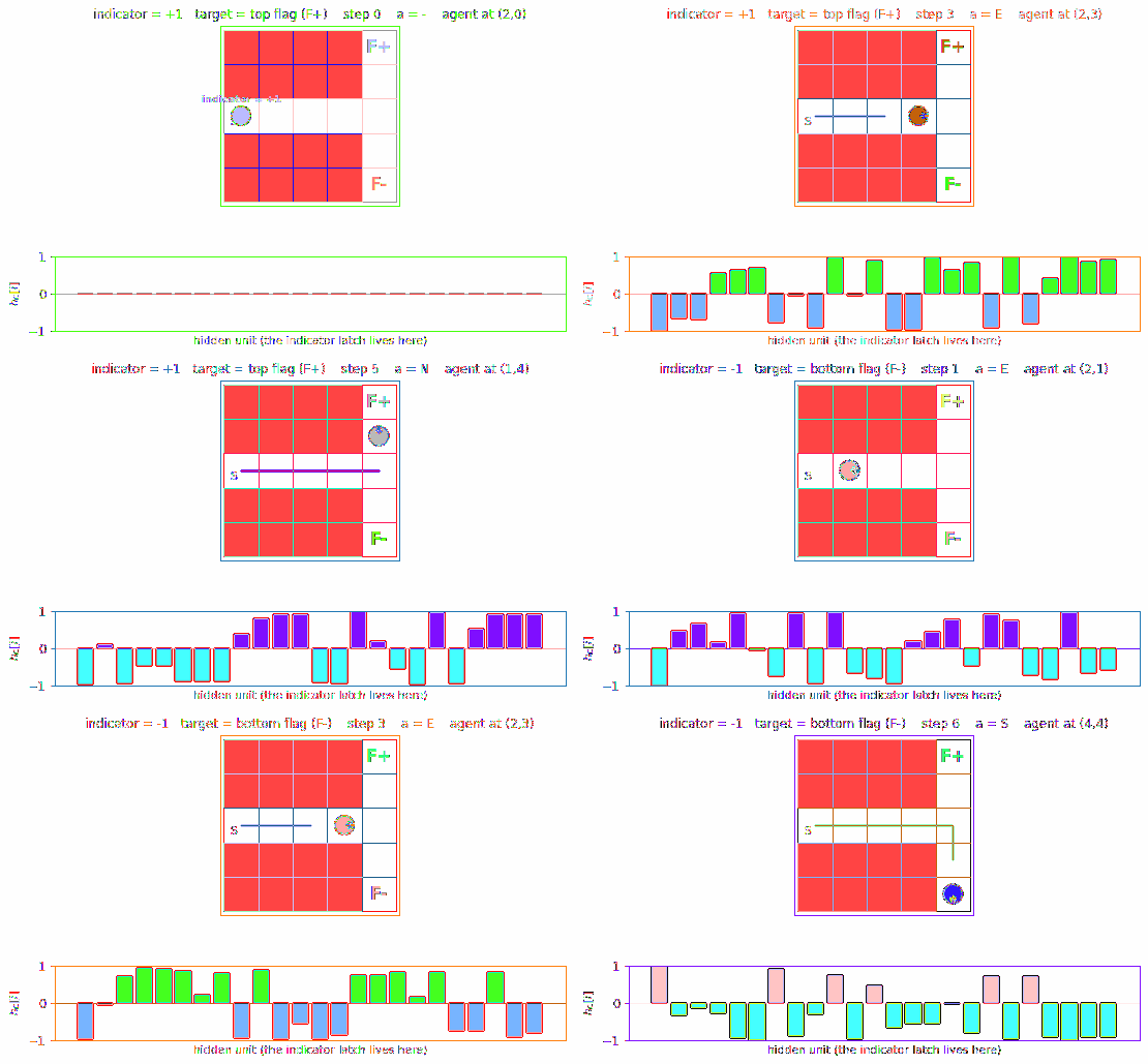
pomdp-flag-maze — pomdp-flag-maze Schmidhuber (1991), Reinforcement learning in Markovian and non-Markovian environments A 2-D T-maze with a hidden flag. The agent observes only its local 4-wall context plus a 1-bit indicator that is non-zero ONLY at the start cell. Recurrent M+C architecture must latch the indicator across the full episode.

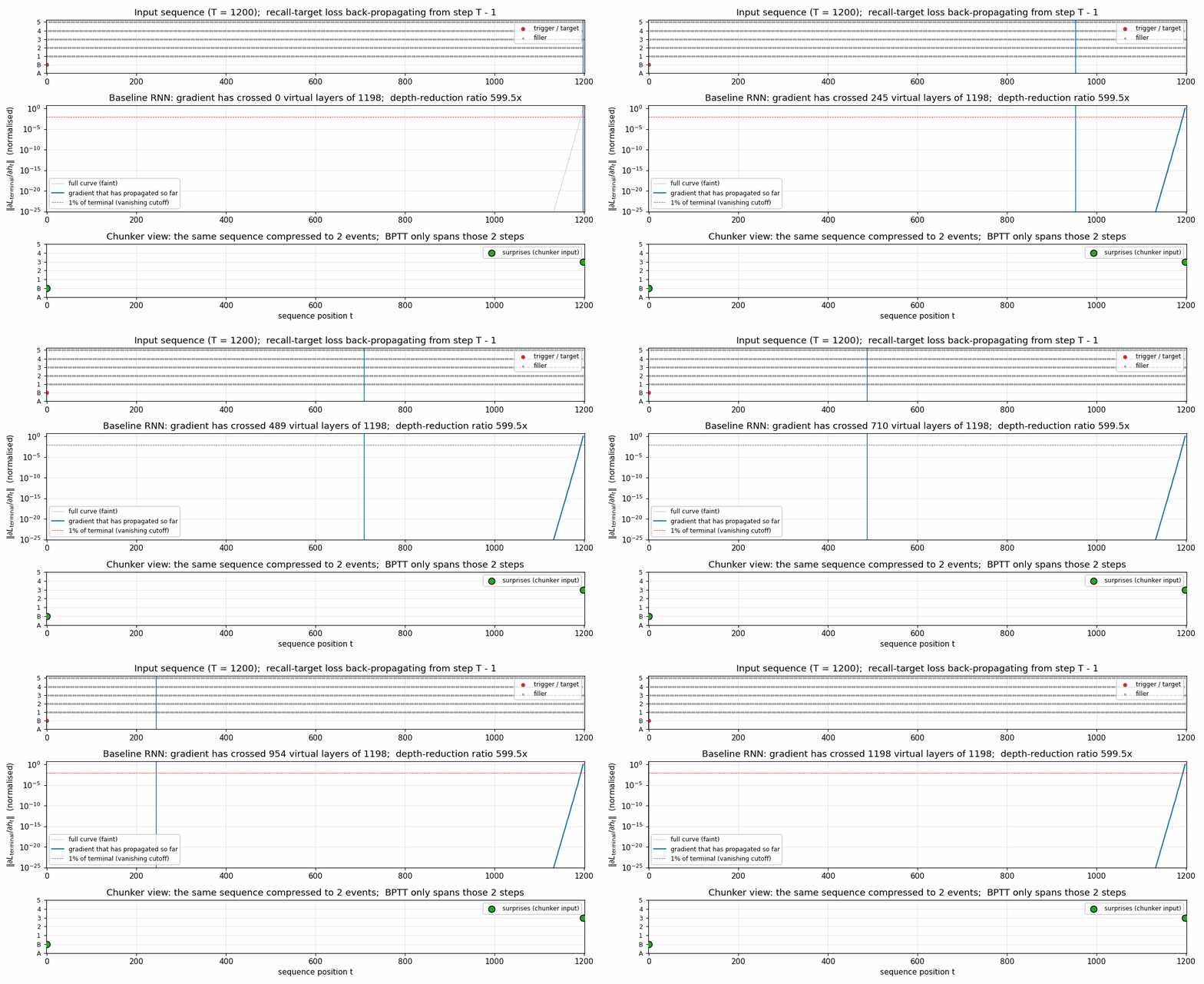
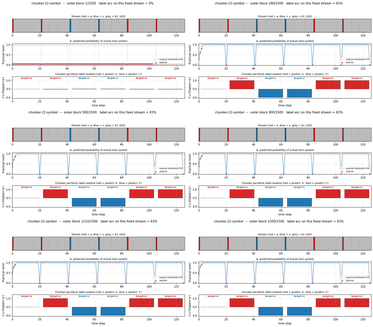
chunker-22-symbol — chunker-22-symbol Schmidhuber (1991/1992), Neural sequence chunkers 22-symbol alphabet streamed without episode boundaries. Two-network history compression: automatizer A predicts next symbol; chunker C only receives A's prediction failures (surprises). The 20-step lag bridge that vanilla BPTT/RTRL fails on.

1992, Neural Computation triple

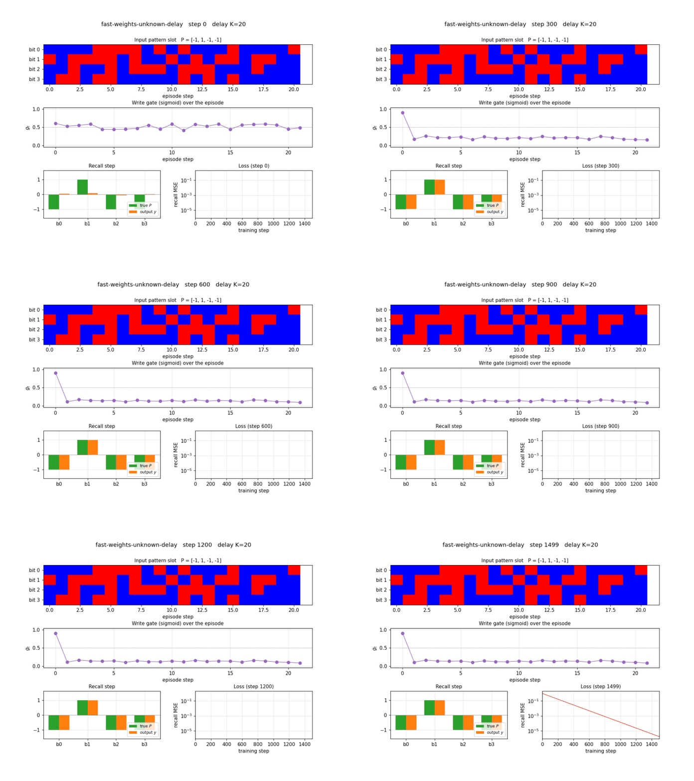
fast-weights-unknown-delay — fast-weights-unknown-delay Schmidhuber (1992), Learning to control fast-weight memories Two arbitrary input signals must be associated across a time gap of unknown length. Slow programmer net S (917 params, 4 heads: key/value/query/gate); W_fast updated as W_fast += eta · g_t · outer(v_t, k_t).

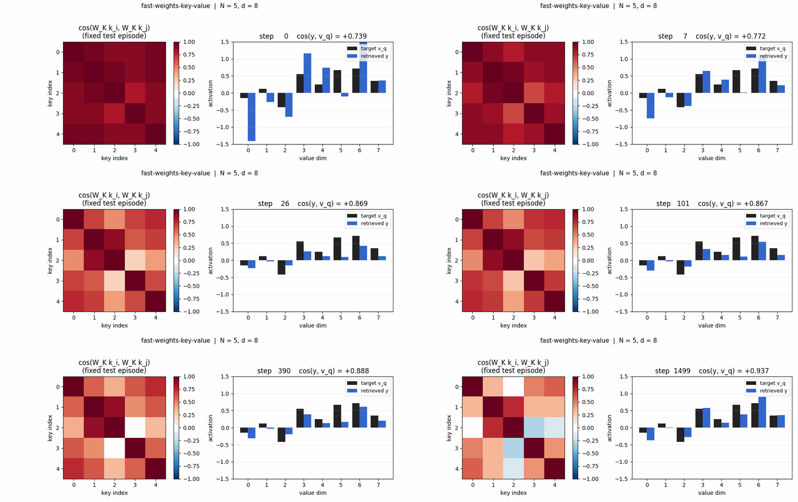
fast-weights-key-value — fast-weights-key-value Schmidhuber (1992), Learning to control fast-weight memories A sequence of (key, value) pairs is presented one step at a time. Each step writes an outer-product update into a fast weight matrix. Retrieval = W_fast · k_query.

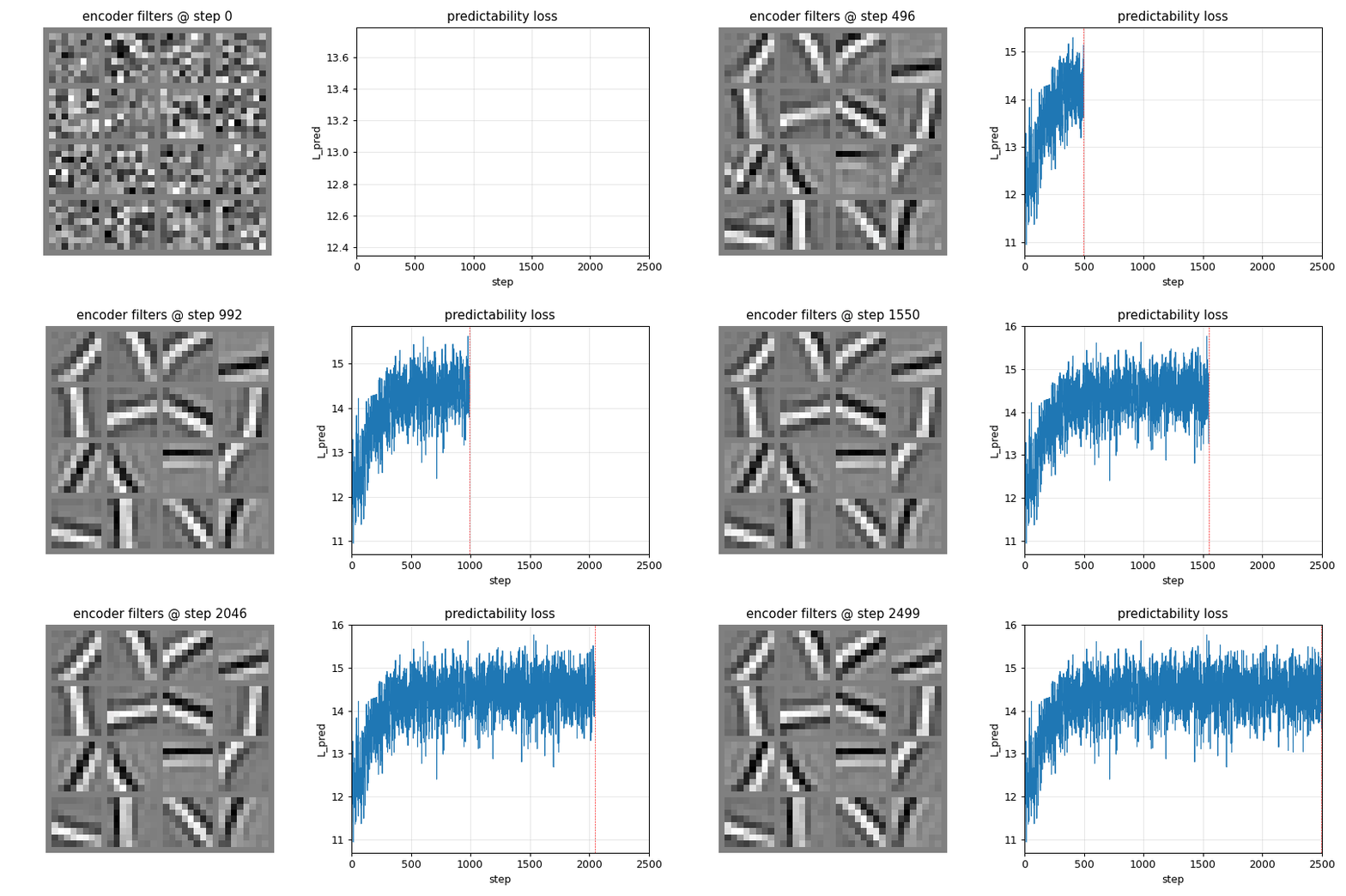
predictability-min-binary-factors — predictability-min-binary-factors Schmidhuber (1992), Learning factorial codes by predictability minimization Given an observable x produced by a fixed random linear mixing of K independent binary factors, learn an encoder E: x to y that produces a factorial code. Adversarial setup: encoder maximizes per-component predictor MSE; predictors minimize it.

1993, Predictable classifications, self-reference, very deep chunking

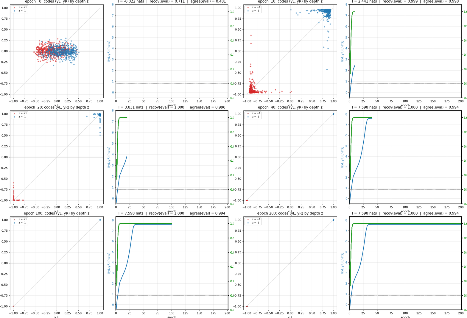
predictable-stereo — predictable-stereo Schmidhuber & Prelinger (1993), Discovering predictable classifications Predictability maximization, the dual of PM. Two networks each see one view of the same synthetic stereo scene; their job is to produce scalar codes that maximally agree.

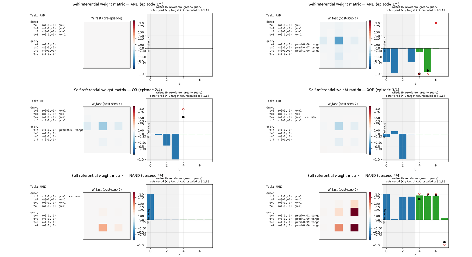
self-referential-weight-matrix — self-referential-weight-matrix Schmidhuber (1993), A self-referential weight matrix A recurrent network whose weight matrix is itself part of the state. W_eff = W_slow + W_fast. Slow params trained by BPTT across episodes; fast plastic matrix is reset each episode and rewritten by the network's own outputs every step.

chunker-very-deep-1200 — chunker-very-deep-1200 Schmidhuber (1993), Habilitationsschrift The Habilitationsschrift's "very deep learning" demonstration: the two-network neural sequence chunker doing credit assignment over roughly 1200 unrolled time-steps. Effective BPTT depth T - 1 = 1199 (raw) compresses to 2 (chunker on surprises).

1995-1997, Levin search and the LSTM benchmark suite

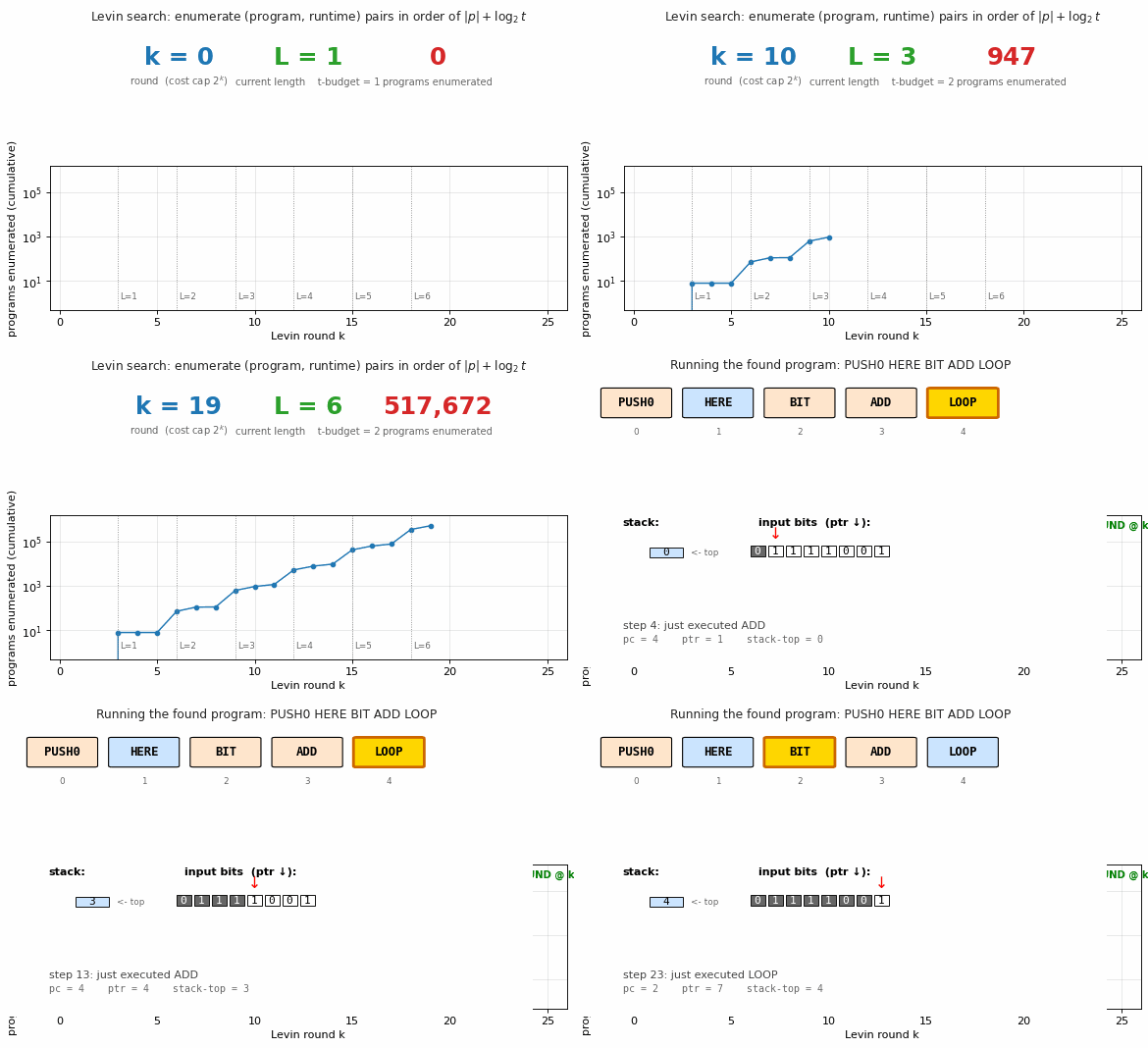
levin-count-inputs — levin-count-inputs Schmidhuber (1995/1997), Discovering solutions with low Kolmogorov complexity Find a program that maps a 100-bit input to its popcount from only 3 training examples, without gradient descent. Levin search enumerates programs ordered by len(p) + log(t). Found program: 5-instr PUSH0 HERE BIT ADD LOOP.

levin-add-positions — levin-add-positions Schmidhuber (1995/1997), Discovering solutions with low Kolmogorov complexity Same Levin enumeration, different target: index-sum of the bit positions where the input is 1 (induces the linear weight vector w_i = i). Found program: length-3 im+. 58 evaluations to find; 200/200 generalize on held-out.

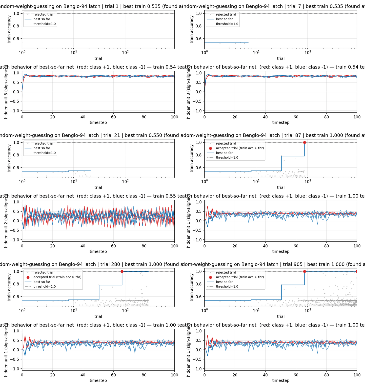
rs-two-sequence — rs-two-sequence Hochreiter & Schmidhuber (1996), LSTM can solve hard long time lag problems Bengio-94 latch task. Random-weight-guessing on a small fully-recurrent net solves what BPTT/RTRL fails on. The point is the algorithm: just sample weights uniformly, run forward, score. No mutation, no crossover, no gradient.

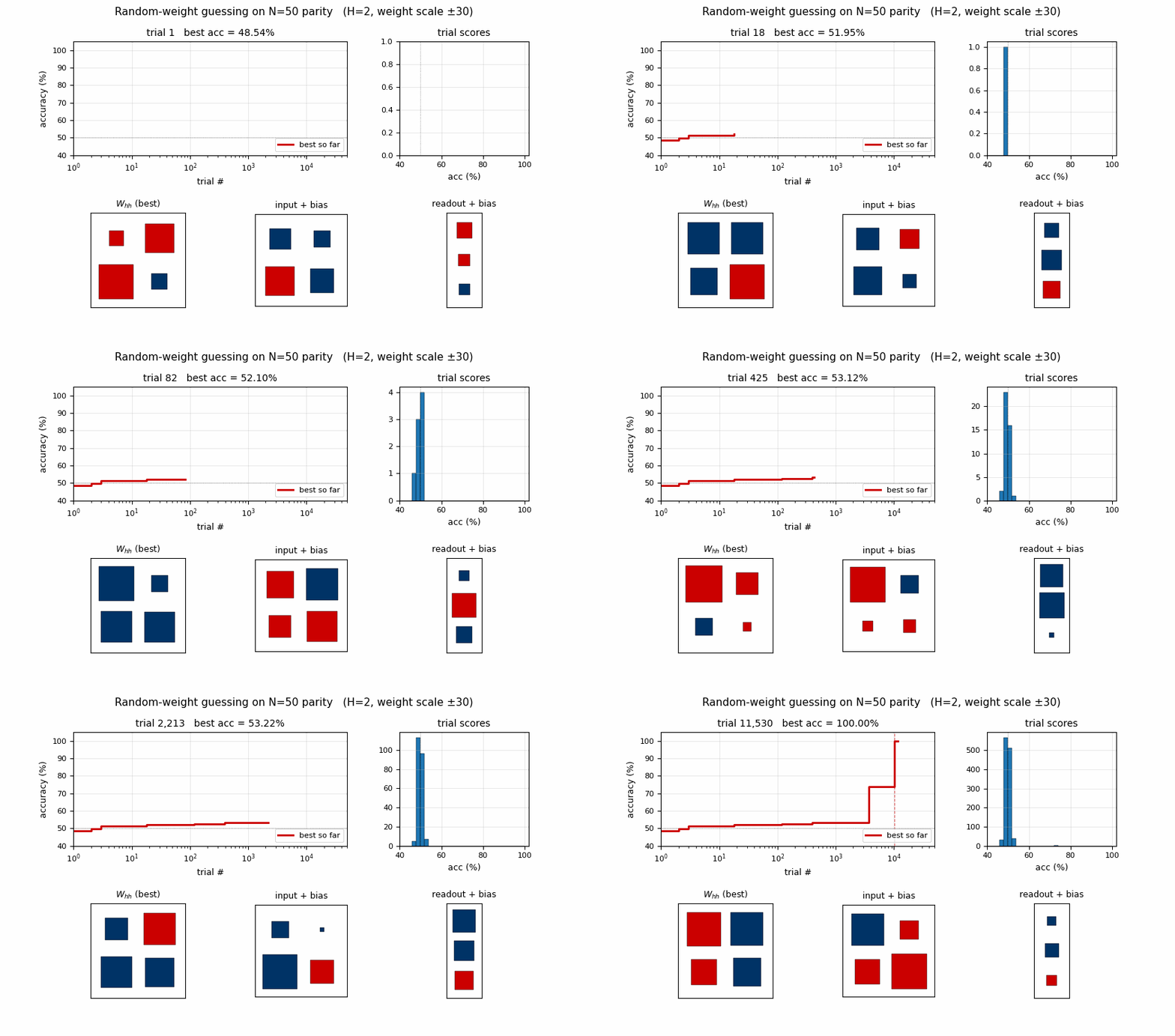
rs-parity — rs-parity Hochreiter & Schmidhuber (1996), LSTM can solve hard long time lag problems N-bit sequence parity (XOR of all input bits) by random weight guessing on a small recurrent net. The parity solution lives in a narrow weight-space basin RS happens to hit by chance. N=50 seed 0: 10,253 trials / 15.3s;

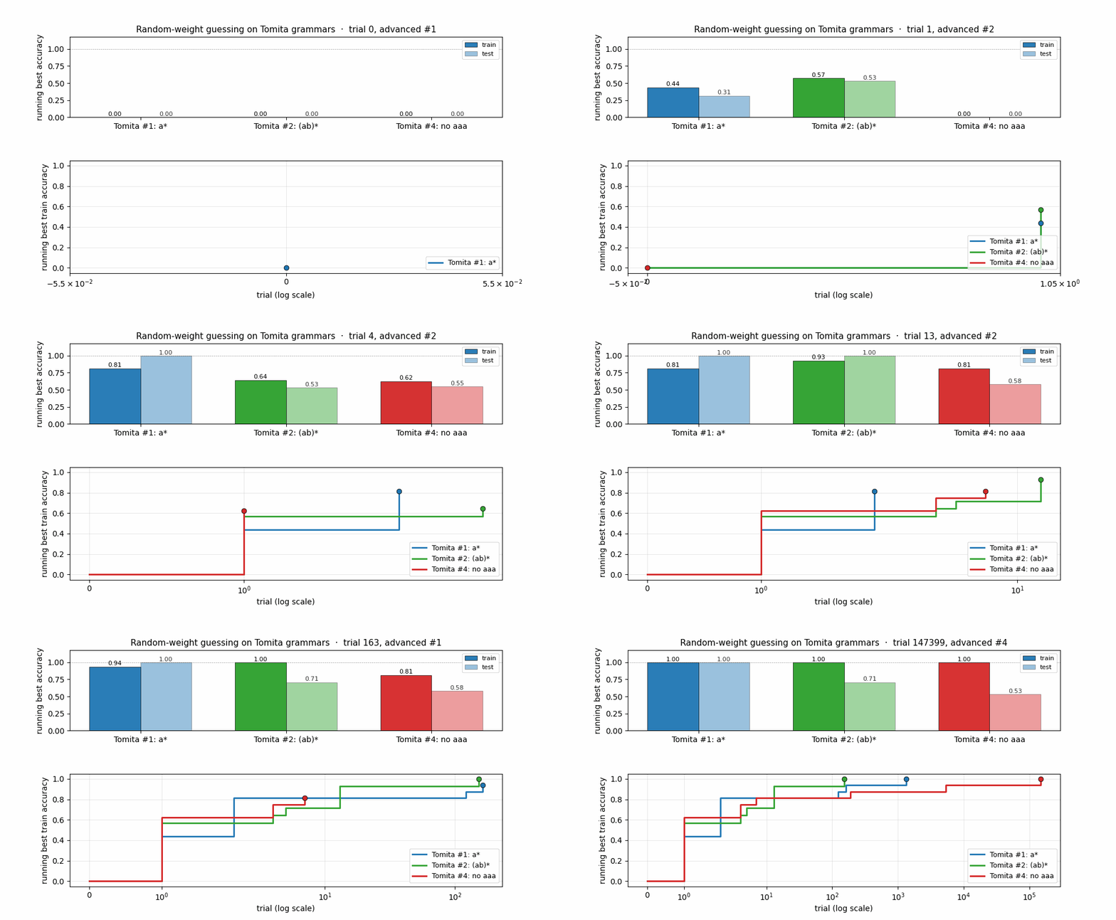
rs-tomita — rs-tomita Hochreiter & Schmidhuber (1996), LSTM can solve hard long time lag problems Random-weight guessing on Tomita grammars #1 (a), #2 ((ab)), and #4 (no aaa substring). Three regular languages of increasing difficulty. All 3 grammars solved across 10 seeds; trial counts within ~3× of paper for #1/#2, ~6× for #4.

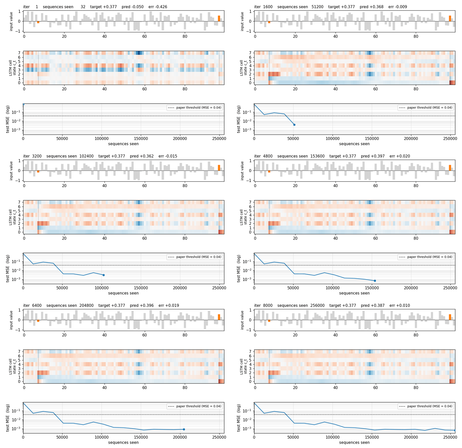
adding-problem — adding-problem Hochreiter & Schmidhuber (1997), Long Short-Term Memory canonical battery T=100 sequences with 2-D inputs: random reals + sparse markers. Target = sum of the 2 marked values. The first non-trivial LSTM benchmark. LSTM MSE 0.0007 (50× under paper's 0.04 threshold); vanilla RNN MSE 0.0706 (gradient vanishes);

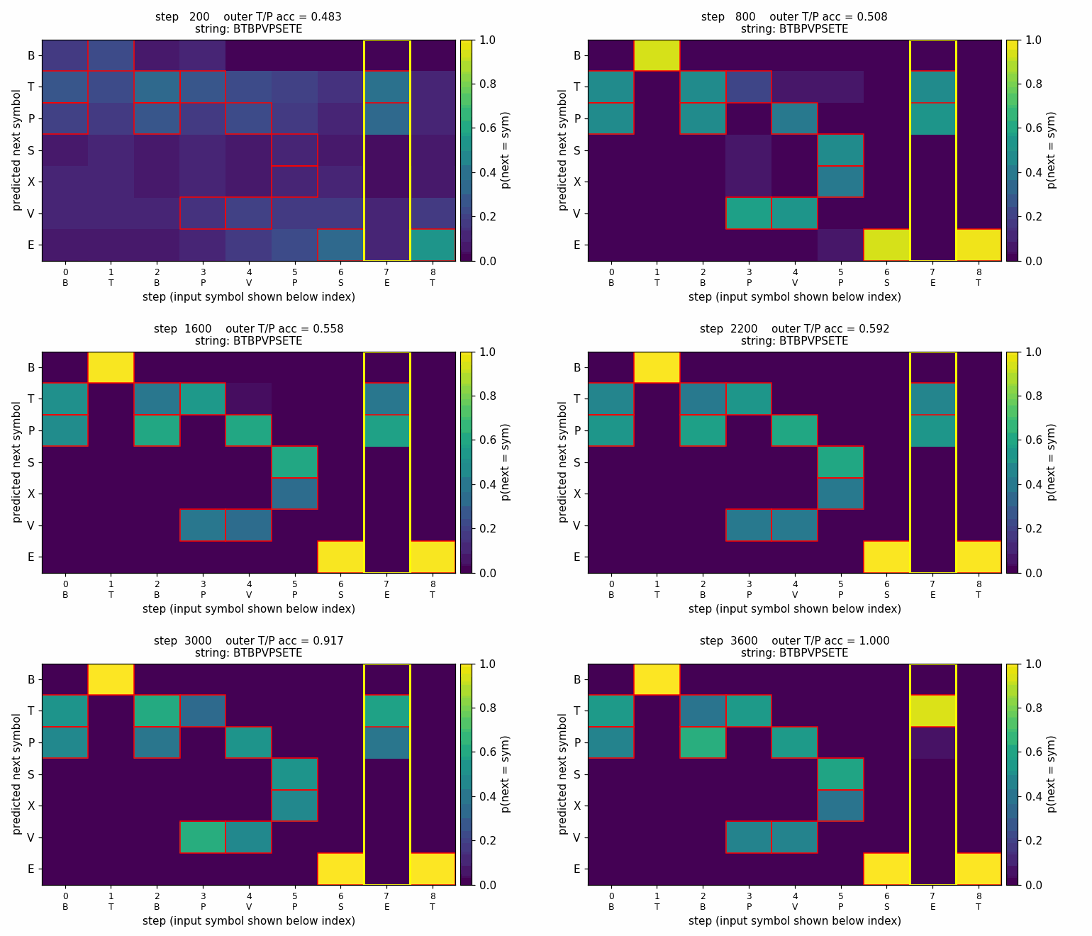
embedded-reber — embedded-reber Hochreiter & Schmidhuber (1997), Long Short-Term Memory canonical battery Reber grammar wrapped with outer T/P matching pair (long-range dependency). Original 1997 LSTM (input + output gate, no forget gate). 10/10 seeds, mean 4800 sequences vs paper 8440-1.8× faster with Adam + negative gate-bias init.

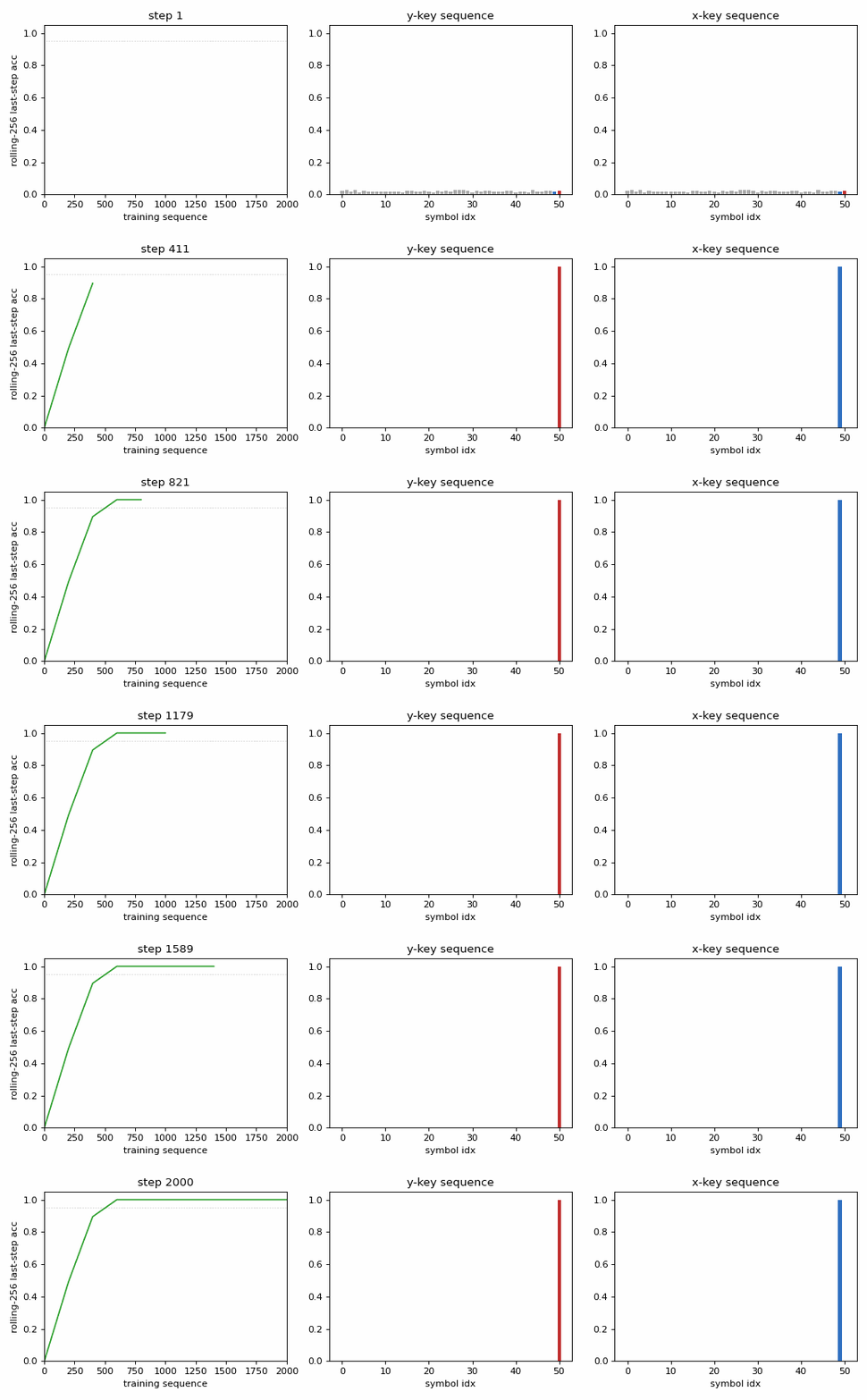
noise-free-long-lag — noise-free-long-lag Hochreiter & Schmidhuber (1997), Long Short-Term Memory canonical battery Two locally-encoded sequences (y, a₁,...,a_{p−1}, y) and (x, a₁,...,a_{p−1}, x). Sub-variant (a) at p=50: solved at sequence 600.

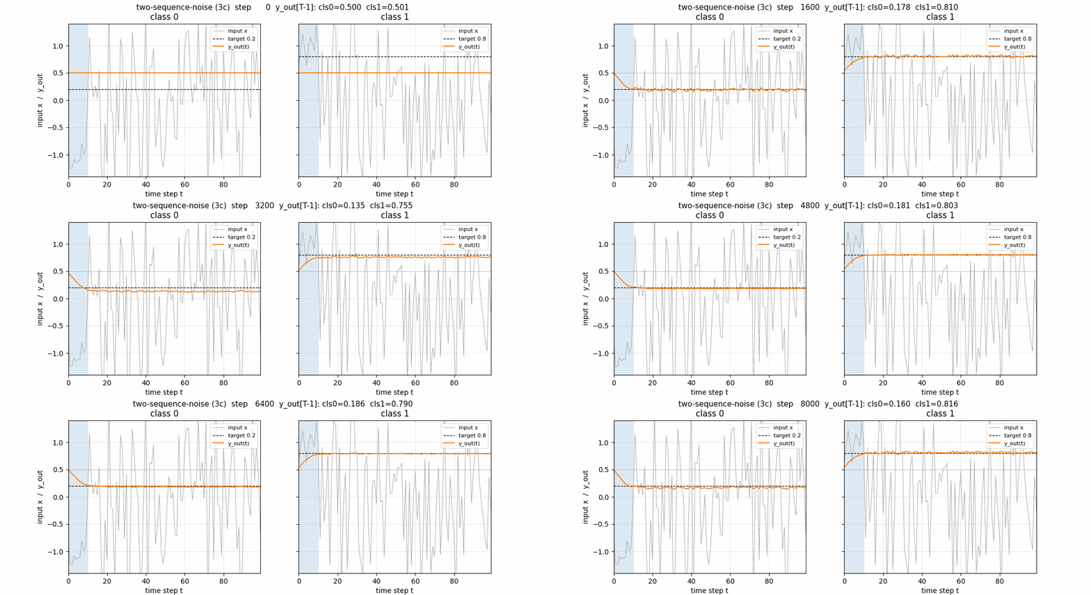
two-sequence-noise — two-sequence-noise Hochreiter & Schmidhuber (1997), Long Short-Term Memory canonical battery Variant 3c (target noise σ=0.32). Canonical 1997 LSTM, 3 blocks × 2 cells = 6 cells, 103 params. Output-gate biases per block = -2, -4, -6 (paper's recipe). 4/4 seeds 100% accuracy on noiseless test sequences.

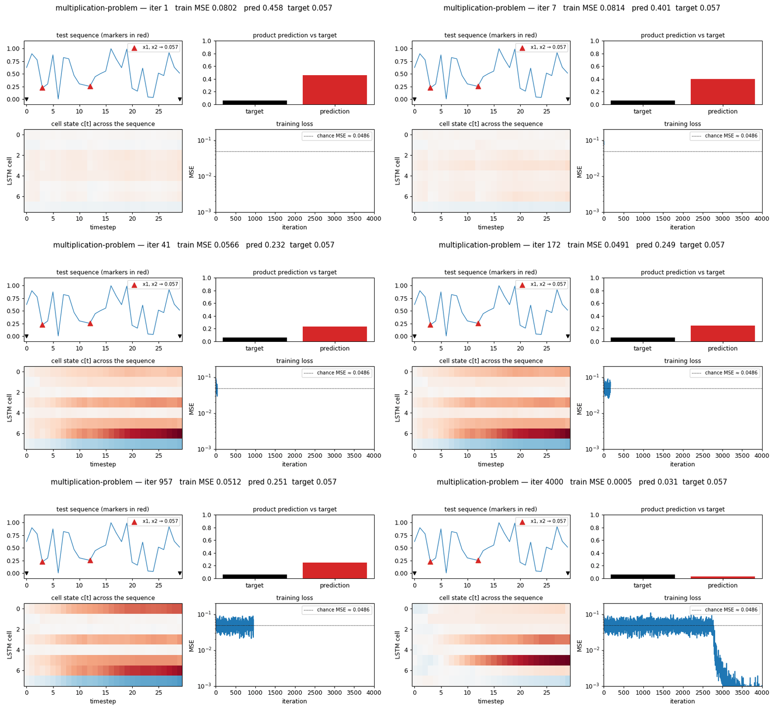
multiplication-problem — multiplication-problem Hochreiter & Schmidhuber (1997), Long Short-Term Memory canonical battery Same as adding-problem but target = product of the 2 marked values. LSTM with forget gate (Gers 2000). MSE 0.0028 at T=30 (17× chance); 3/5 seeds converge, paper-faithful per-seed brittleness.

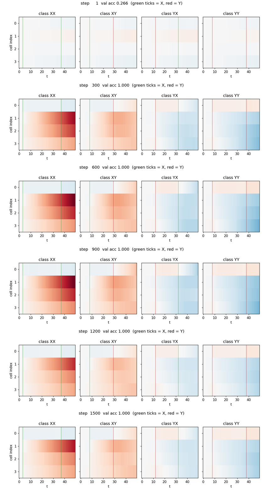
temporal-order-3bit — temporal-order-3bit Hochreiter & Schmidhuber (1997), Long Short-Term Memory canonical battery Two information-carrying symbols X, Y at unknown positions; classify the temporal order (XX, XY, YX, YY). Original 1997 LSTM (no forget gate). 5/5 seeds 100%, median ~6.4k seqs vs paper 31,390 (Adam advantage). Vanilla RNN at chance 0.25.

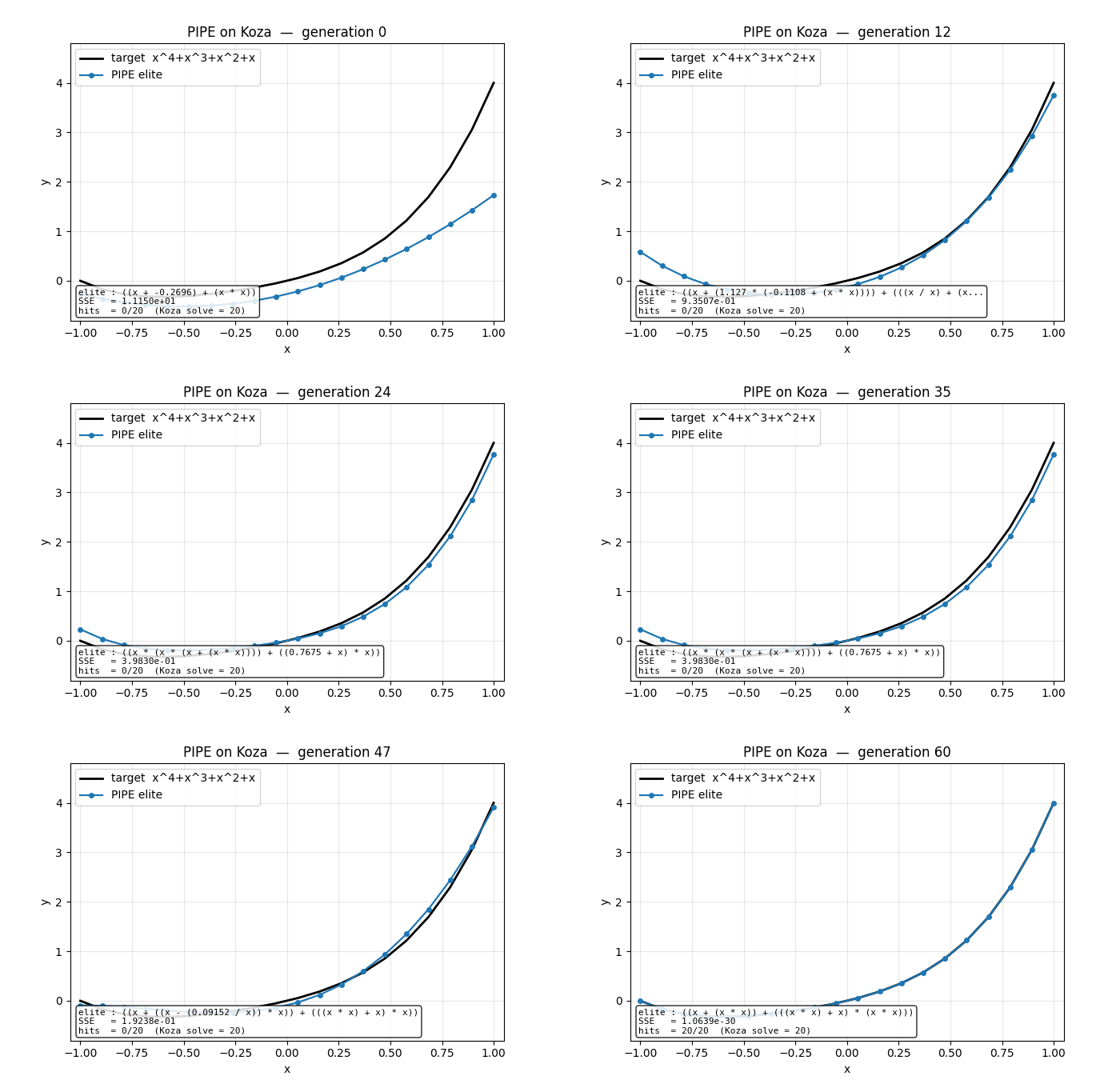
pipe-symbolic-regression — pipe-symbolic-regression Salustowicz & Schmidhuber (1997), Probabilistic Incremental Program Evolution Symbolic regression on Koza's classic benchmark f(x) = x⁴ + x³ + x² + x. Probabilistic Prototype Tree (PPT) over {+, −, *, /, x, R}. PBIL update toward elite at every visited node; per-component mutation along elite path. No gradient, no crossover.

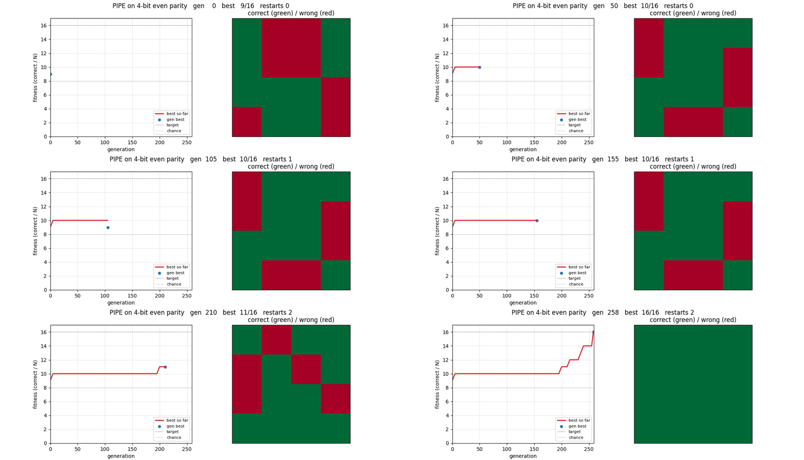
pipe-6-bit-parity — pipe-6-bit-parity Salustowicz & Schmidhuber (1997), Probabilistic Incremental Program Evolution Same PIPE machinery on Boolean function set {AND, OR, NOT, IF, x_0..x_5}. Bitmask program evaluator runs all 64 inputs in O(tree_size) bitwise ops. 4-bit even parity solves cleanly at gen 258 (16/16); 6-bit reaches 71.9% at the 240s budget cap.

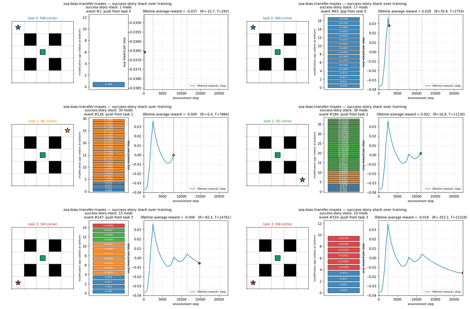
ssa-bias-transfer-mazes — ssa-bias-transfer-mazes Schmidhuber, Zhao, Wiering (1997), Shifting inductive bias with SSA Success-story algorithm: keep a stack of policy modifications; only retain modifications that produce statistically significant lifetime-reward improvements (history-conditioned, not per-task). Bias from one task transfers to the next.

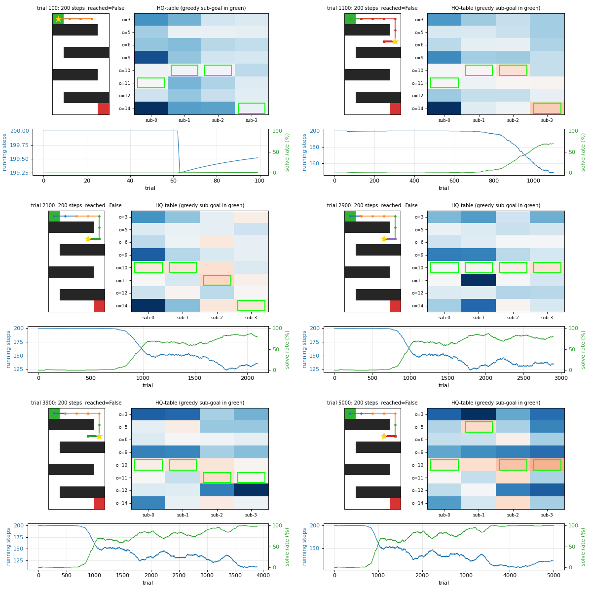
hq-learning-pomdp — hq-learning-pomdp Wiering & Schmidhuber (1997), HQ-learning Hierarchical Q(λ) for POMDP. M sub-agents with their own Q-tables; control transfers between sub-agents at sub-goal observations. Honest non-replication: paper's HQ-vs-flat gap doesn't reproduce on the 29-cell maze.

semilinear-pm-image-patches — semilinear-pm-image-patches Schmidhuber, Eldracher, Foltin (1996), Semilinear PM Linear encoder y = Wx on the Stiefel manifold (polar projection after every step). Predictor input is the standardised squared code z = (y² - μ) / σ (the squaring is the one nonlinearity, "semilinear").

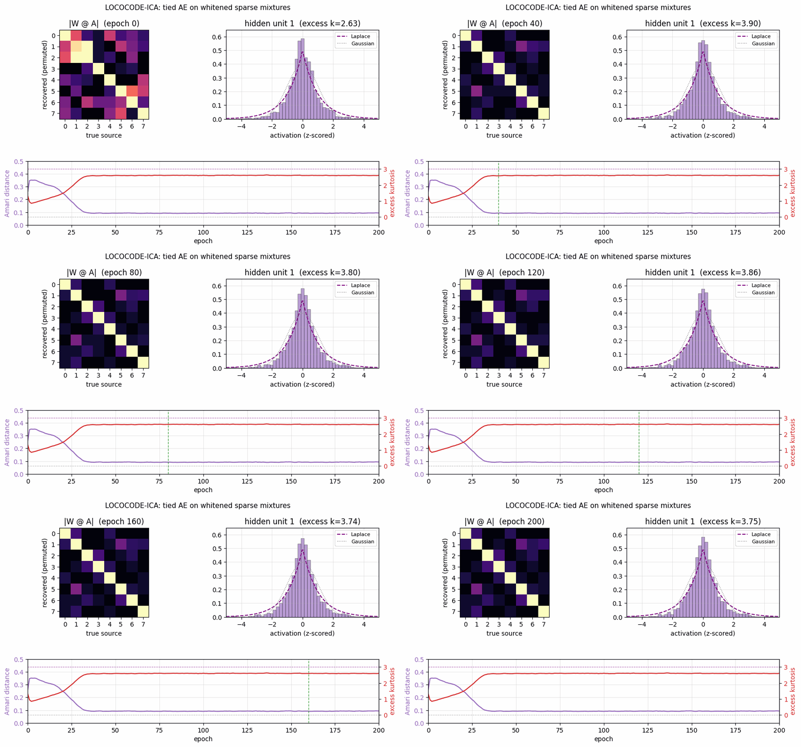
lococode-ica — lococode-ica Hochreiter & Schmidhuber (1999), LOCOCODE Tied autoencoder + L1 sparsity on whitened input (surrogate for the paper's flat-minimum-search Hessian penalty). On synthetic Laplacian sources: Amari distance 0.093-4× better than PCA (0.388), within 5× of FastICA (0.022).

2000-2002, LSTM follow-ups

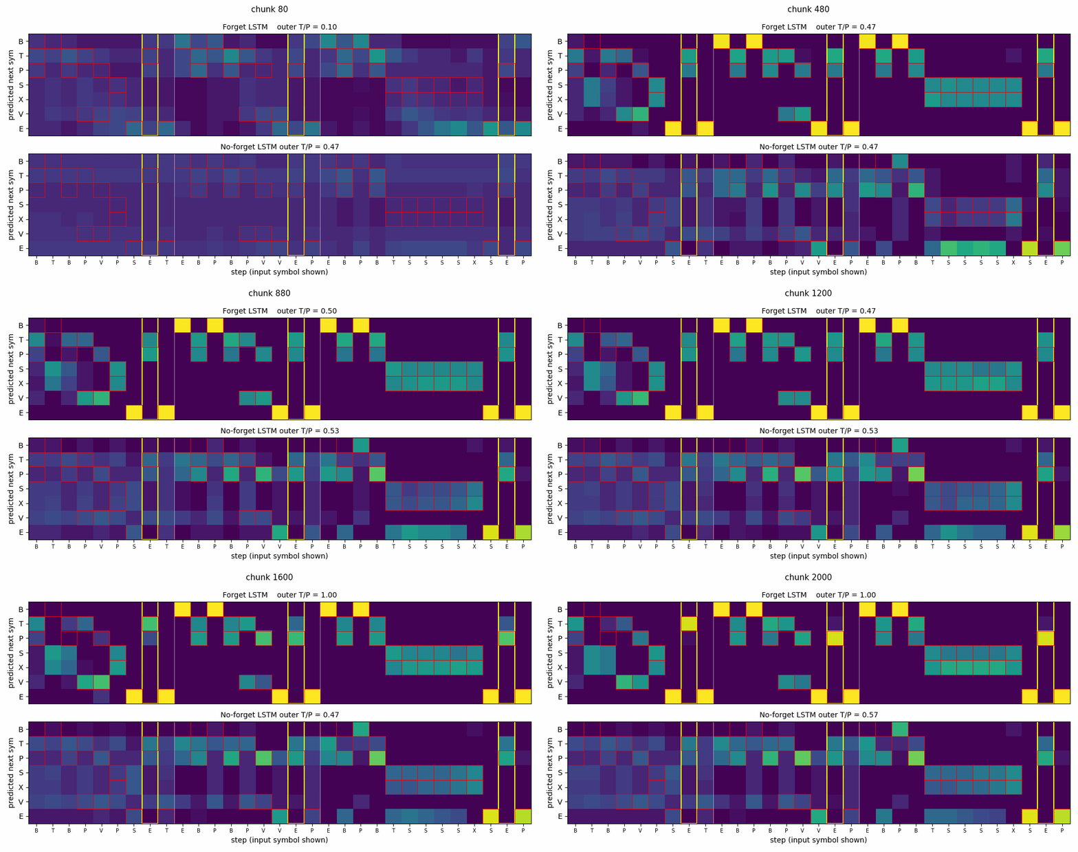
continual-embedded-reber — continual-embedded-reber Gers, Schmidhuber, Cummins (2000), Learning to forget Embedded Reber strings concatenated without any episode reset. Mechanism contrast made visible: forget-gate LSTM cell-state norm stabilizes at ~25; no-forget-gate norm grows to ~295 across the stream. Forget gates drop at end-of-string offsets.

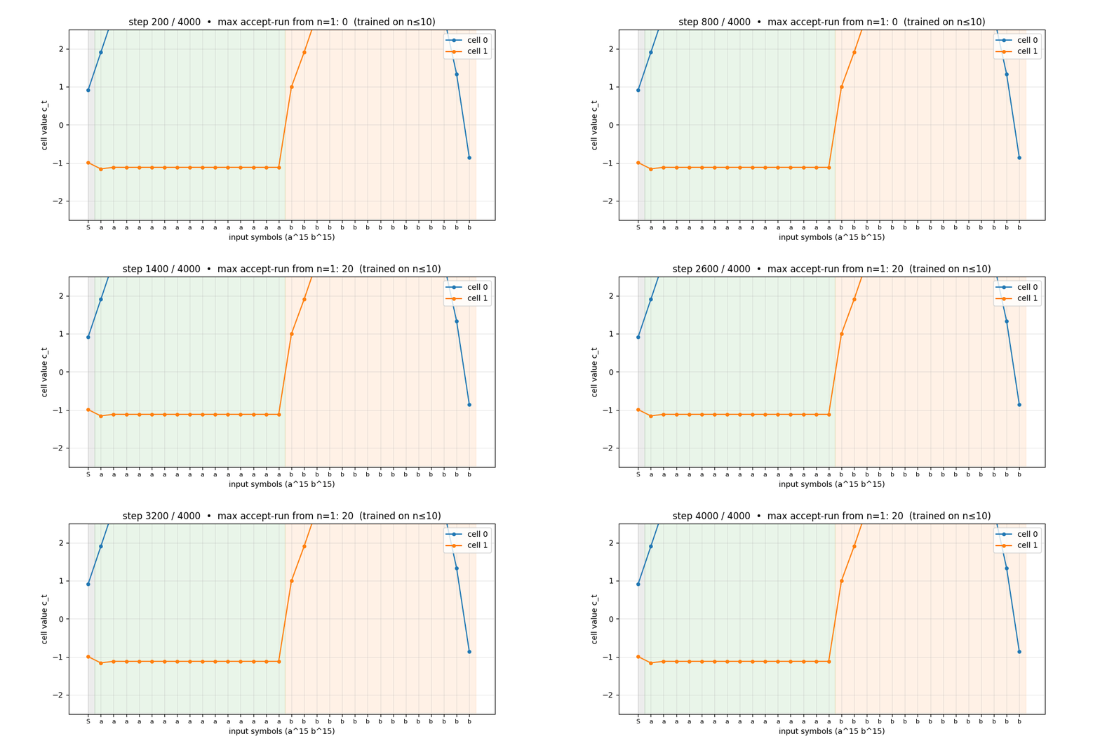
anbn-anbncn — anbn-anbncn Gers & Schmidhuber (2001), Context-free and context-sensitive languages Two formal languages: a^n b^n (context-free) and a^n b^n c^n (context-sensitive). Peephole LSTM (Gers 2002 cell). Cell 0 emerges as a clean linear counter, charges during a's, discharges during b's. Trained n=1..10 to generalizes a^n b^n to n=1..65;

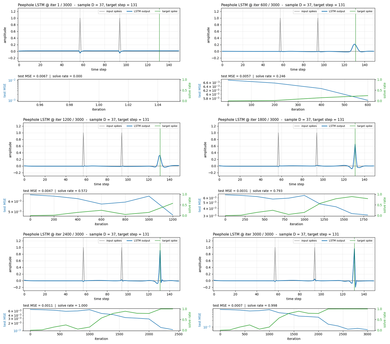
timing-counting-spikes — timing-counting-spikes Gers, Schraudolph, Schmidhuber (2002), Learning precise timing Measure-Spike-Distance (MSD): two input spikes at t1 < t2; network must fire at t1 + 2·(t2 - t1). Peephole LSTM (cell state feeds gates). One cell develops an analog interval timer across the inter-spike gap.

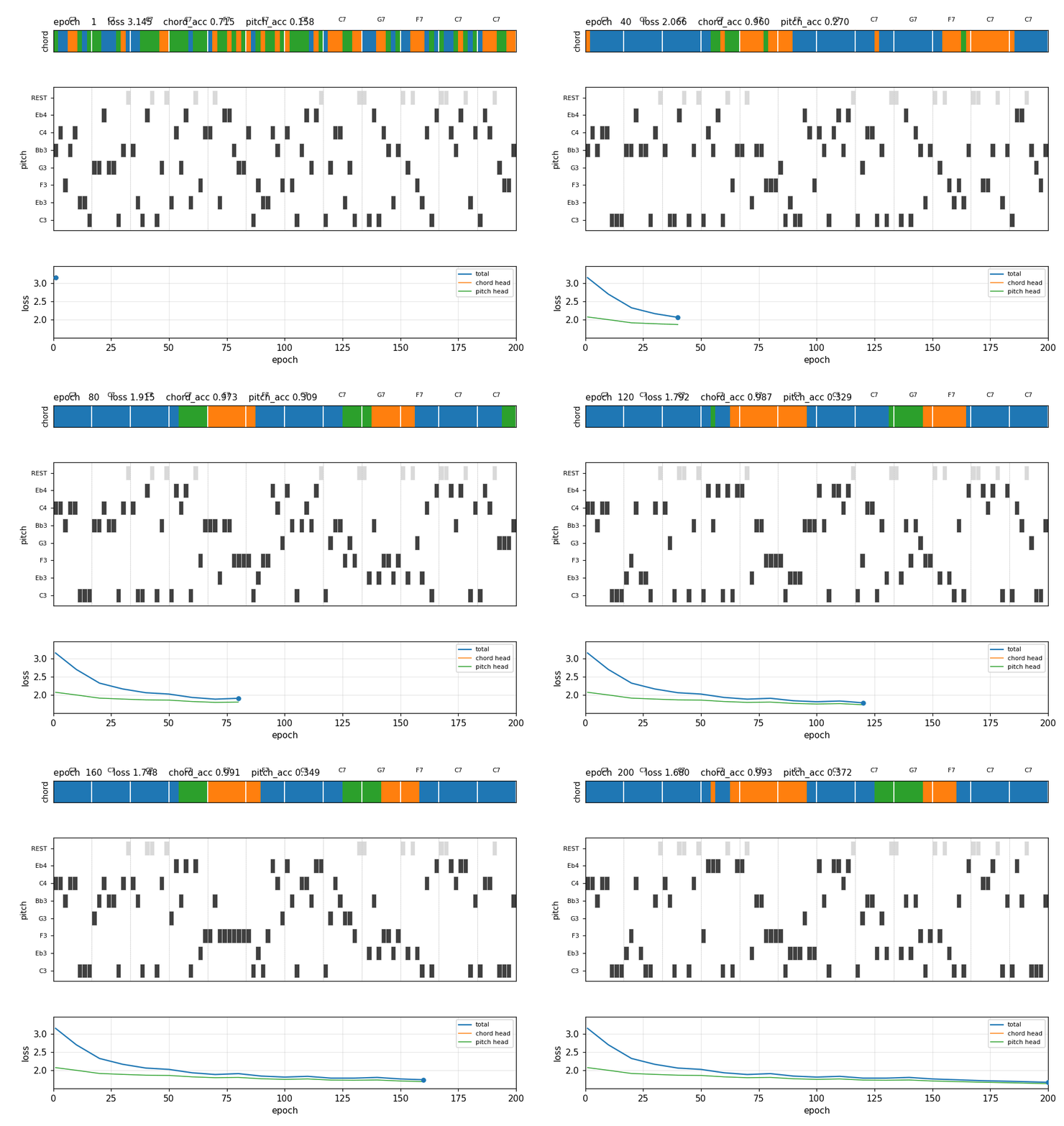
blues-improvisation — blues-improvisation Eck & Schmidhuber (2002), Blues improvisation 12-bar bebop blues. Fixed chord progression: C7 C7 C7 C7 / F7 F7 C7 C7 / G7 F7 C7 C7. 2-layer stacked LSTM (chord layer H1=20 to melody layer H2=24). 8 hand-synthesized 12-bar choruses (no external MIDI). 12/12 bar-onset chord match;

2002-2010, Evolutionary RL, OOPS, BLSTM+CTC

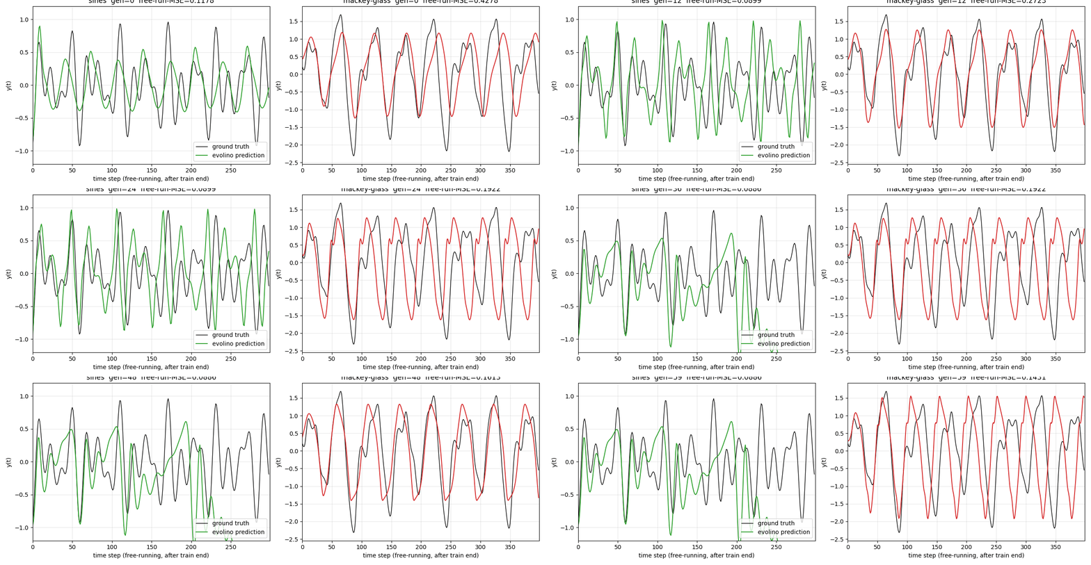
evolino-sines-mackey-glass — evolino-sines-mackey-glass Schmidhuber, Wierstra, Gomez (2005/2007), Evolino Hybrid neuroevolution + linear regression for sequence learning. LSTM hidden weights evolved by population selection + gaussian mutation + crossover;

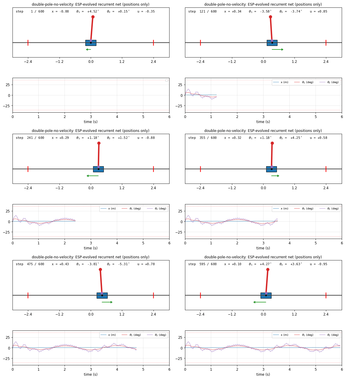
double-pole-no-velocity — double-pole-no-velocity Gomez & Schmidhuber (2005), Co-evolving recurrent neurons Cart with two stacked poles of different lengths (canonical hard non-Markov RL benchmark). Hidden velocities, only positions observed. Wieland 1991 double cart-pole sim in numpy, RK4 integration.

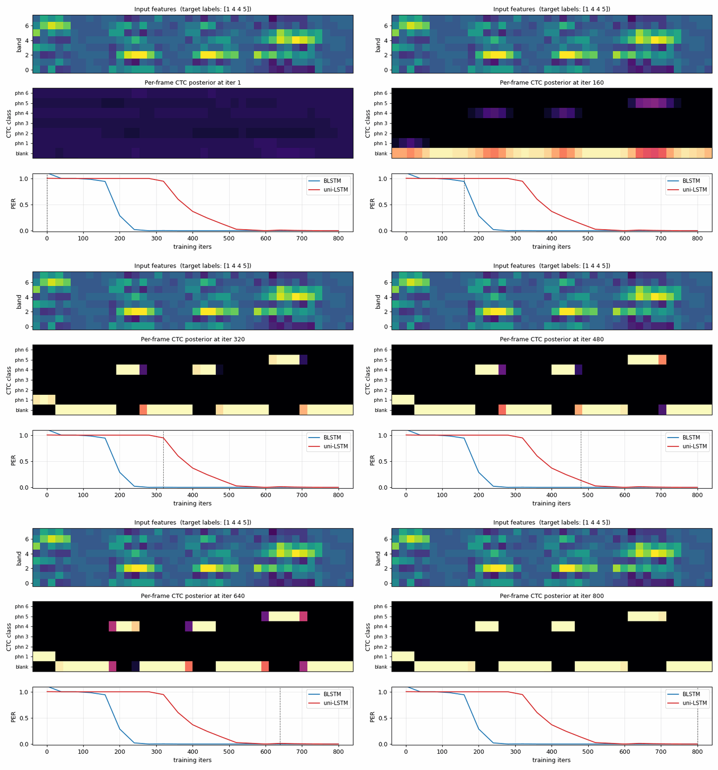
timit-blstm-ctc — timit-blstm-ctc Graves et al. (2005/2006), BLSTM and Connectionist Temporal Classification Synthetic phoneme corpus (K=6 phonemes, 8 mel-like bands, co-articulated shared-onset clusters so future context disambiguates). Bidirectional LSTM + log-space CTC forward-backward. BLSTM 1.87× faster than uni-LSTM (5/5 seeds 300 vs 560 iters);

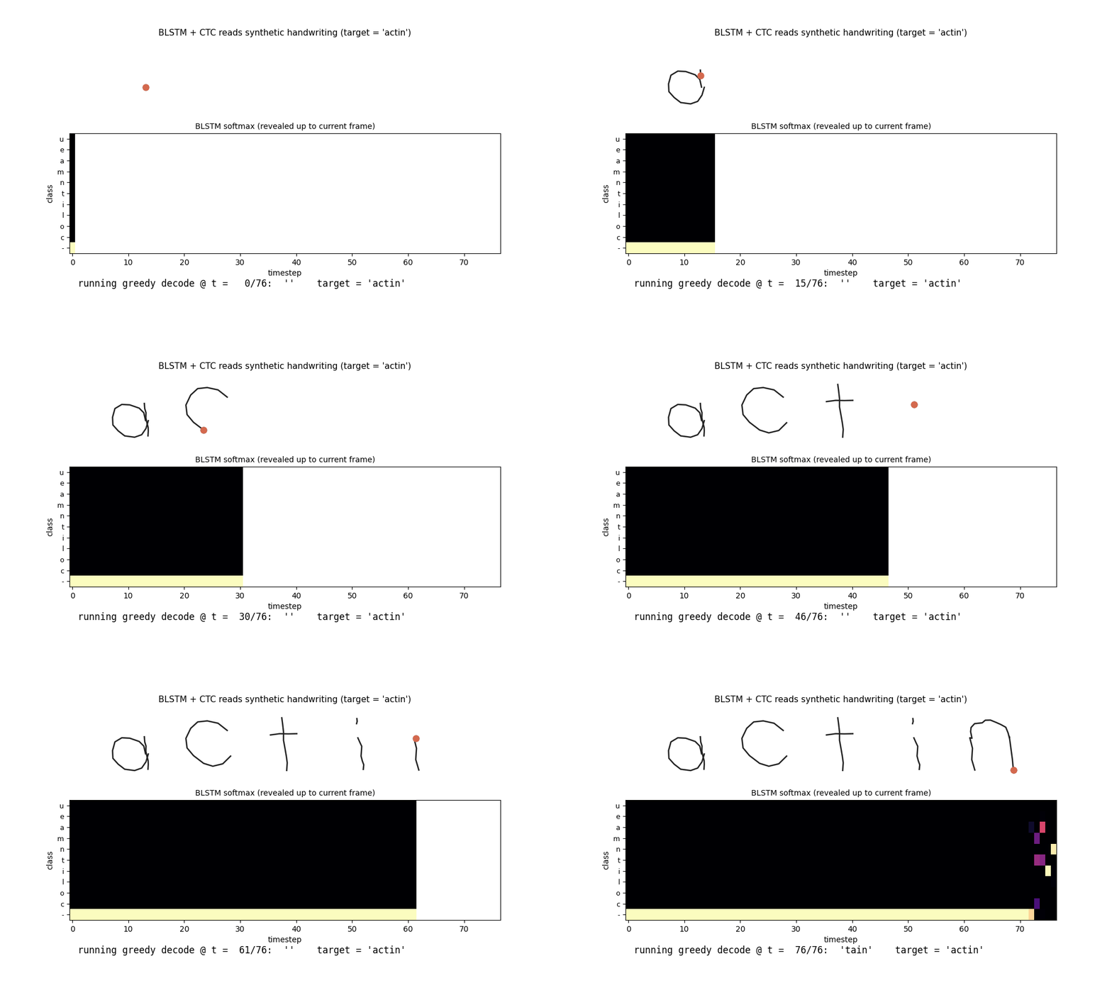
iam-handwriting — iam-handwriting Graves, Liwicki, Fernández, Bertolami, Bunke, Schmidhuber (2009), Unconstrained handwriting 10-character hand-crafted alphabet, each glyph from ellipse arcs + line segments; 47-word vocab; per-word affine slant + per-point Gaussian jitter. BLSTM + CTC reads pen-trajectory data. In-vocab CER 0.082 / word acc 0.77;

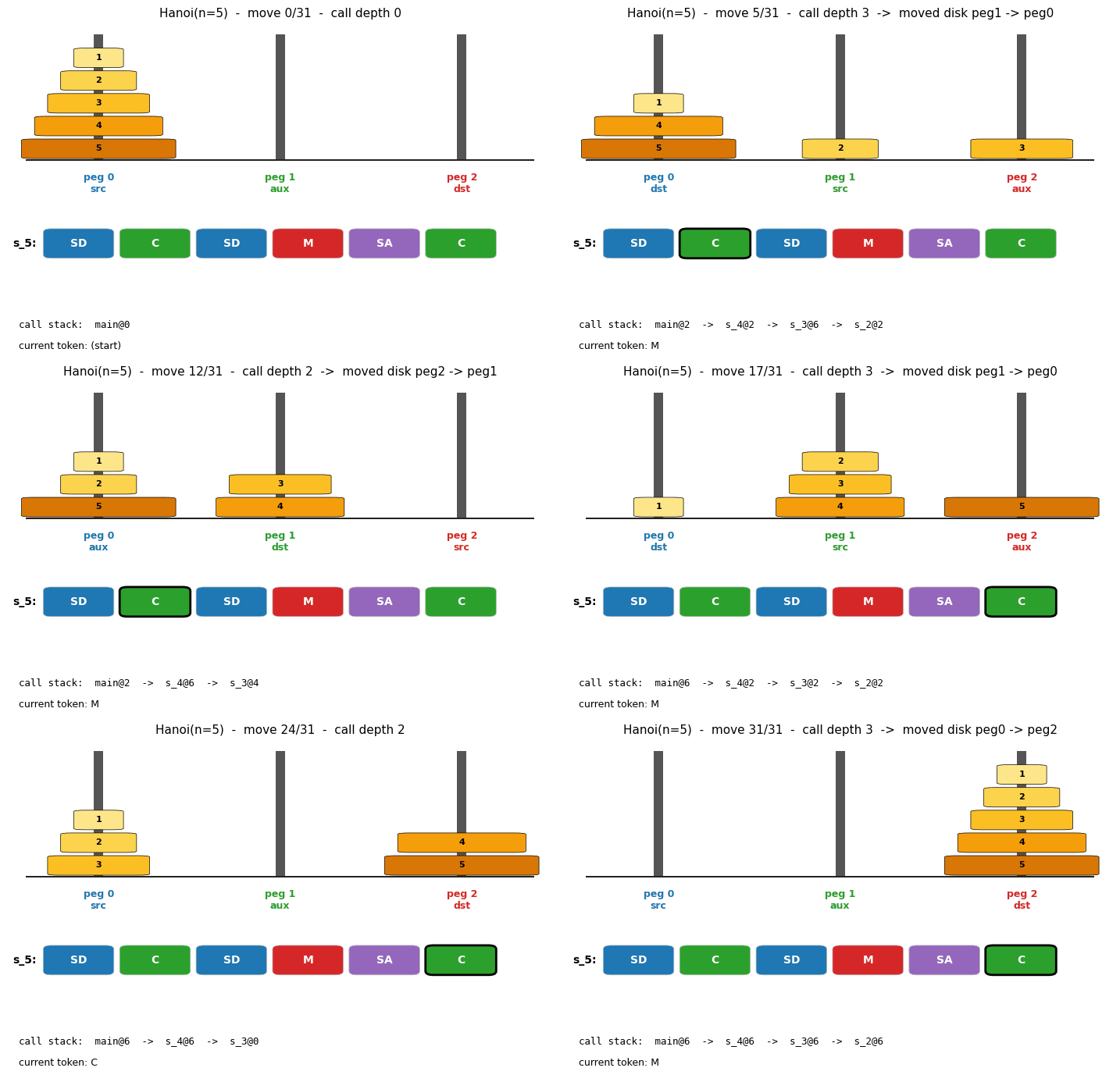
oops-towers-of-hanoi — oops-towers-of-hanoi Schmidhuber (2002-2004), Optimal Ordered Problem Solver Towers of Hanoi: move n disks from peg 0 to peg 2; optimal solution length 2^n - 1. OOPS = Levin search with reusable subroutines. Discovers 6-token recursive solver SD C SD M SA C at n=3; reuses with zero search from n=4 onward.

2010-2017, Deep learning at scale

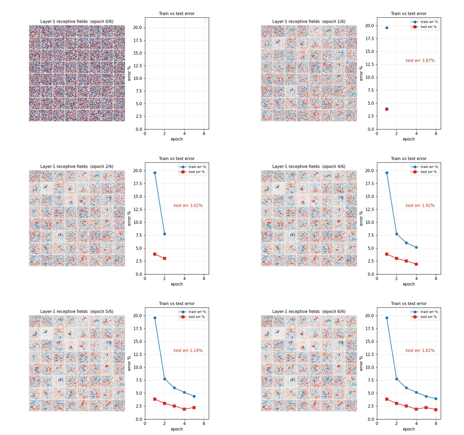
mnist-deep-mlp — mnist-deep-mlp Cireşan, Meier, Gambardella, Schmidhuber (2010), Deep, big, simple nets MNIST classification with a plain feedforward MLP, no convolution, no pretraining, no model averaging, on heavily deformed training data. Per-batch affine + Simard elastic deformation in pure numpy (separable Gaussian + bilinear sampling).

mcdnn-image-bench — mcdnn-image-bench Cireşan, Meier, Schmidhuber (2012), Multi-column DNN Single-column 4-layer ReLU MLP on MNIST (paper's multi-column ensemble + GTSRB/CASIA deferred to v1.5). 1.46% test err; multi-seed mean 1.47% ± 0.03%. Honest gap: paper 35-column ensemble 0.23%, single CNN ~0.4%.

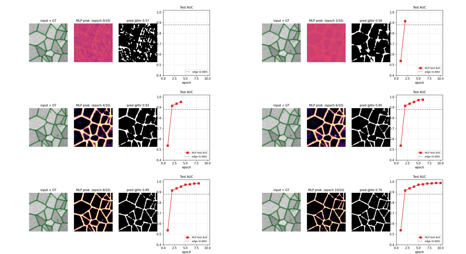
em-segmentation-isbi — em-segmentation-isbi Cireşan, Giusti, Gambardella, Schmidhuber (2012), EM segmentation Synthetic Voronoi-EM substitute for ISBI 2012 stack: random Voronoi tessellation + dark 1-px boundaries + per-cell intensity + Gaussian noise + sparse organelles + 3×3 PSF blur. MLP pixel classifier on 32×32 patches.

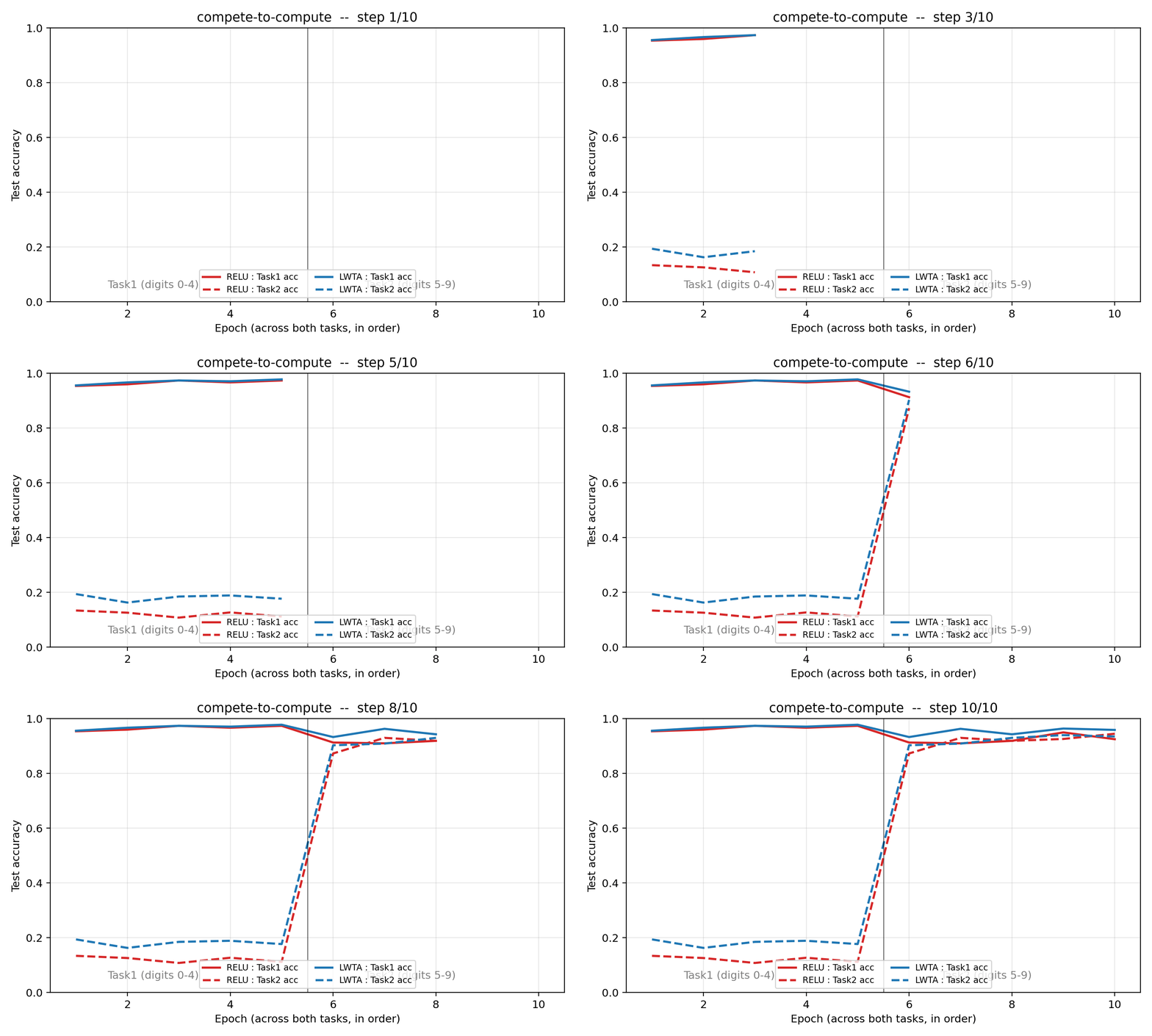
compete-to-compute — compete-to-compute Srivastava, Masci, Kazerounian, Gomez, Schmidhuber (2013), Compete to compute LWTA (Local Winner-Take-All): groups of k=2 units per layer; only the per-group winner forwards activations, others zero out; gradient flows only through the winner. Sequential 2-task MNIST split (digits 0-4 to 5-9).

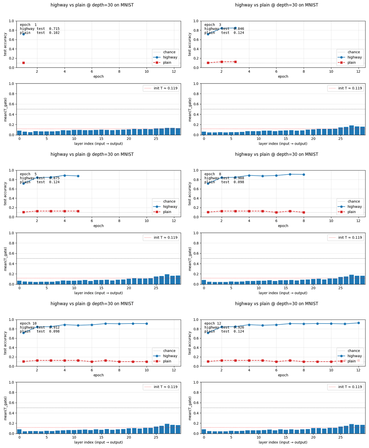
highway-networks — highway-networks Srivastava, Greff, Schmidhuber (2015), Highway Networks Gated deep MLP: y = H(x)·T(x) + x·(1−T(x)) with learned sigmoid gate T. Depth comparison 5/10/20/30/50: highway stable at all depths (0.926 at depth 30); plain MLP dies past depth 10 (stuck at chance 0.124).

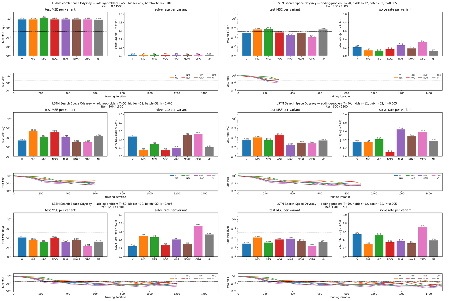
lstm-search-space-odyssey — lstm-search-space-odyssey Greff, Srivastava, Koutník, Steunebrink, Schmidhuber (2017), LSTM Search Space Odyssey 8 LSTM variants in one ablation matrix: V (vanilla), NIG (no input gate), NFG (no forget gate), NOG (no output gate), NIAF (no input activation), NOAF (no output activation), CIFG (coupled input-forget), NP (no peepholes).

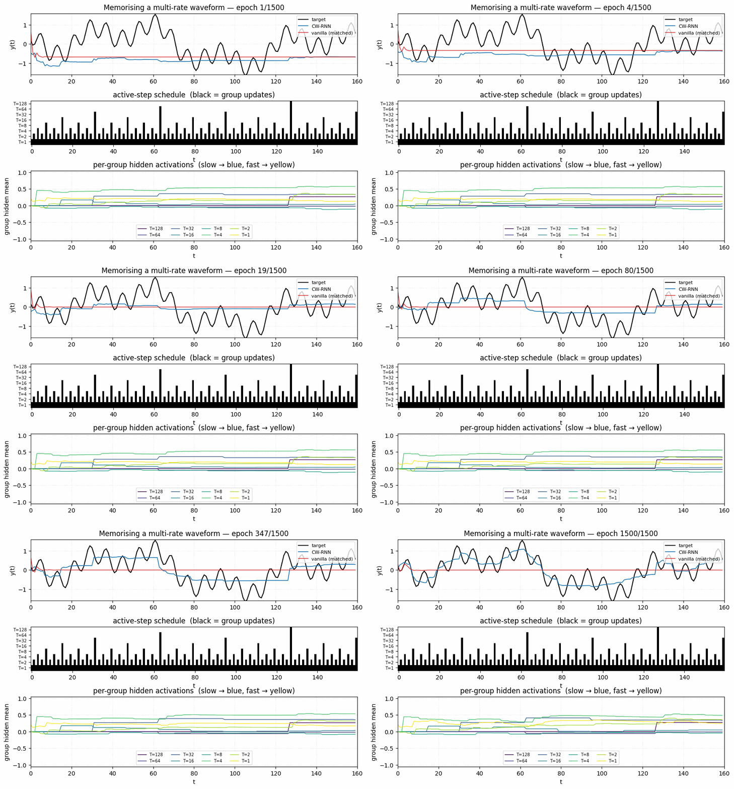
clockwork-rnn — clockwork-rnn Koutník, Greff, Gomez, Schmidhuber (2014), Clockwork RNN Standard Elman RNN with hidden layer partitioned into G modules. Each module g has a clock period T_g; at timestep t a module updates only when t mod T_g == 0. Forward connections only flow from slower clocks to faster clocks.

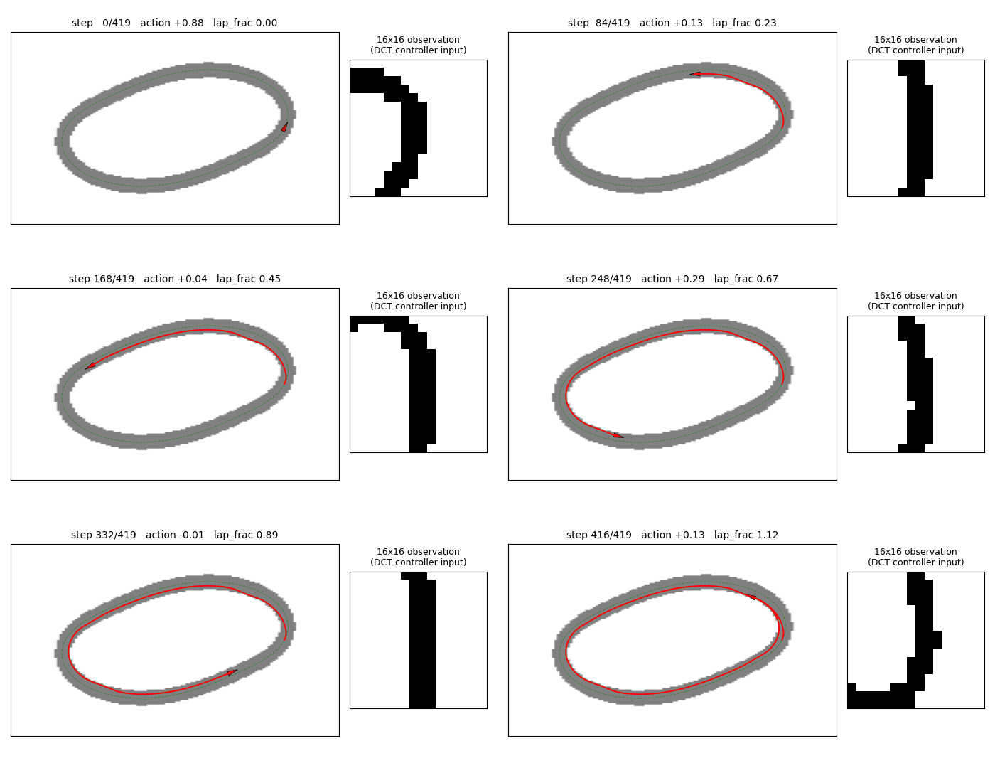
torcs-vision-evolution — torcs-vision-evolution Koutník, Cuccu, Schmidhuber, Gomez (2013), Vision-based RL via evolution Numpy oval racing track + 16×16 pixel observation. MLP 256 to 16 to 1 with W1 parameterized by a 4×4=16 low-frequency 2-D DCT block per hidden unit (decoded via precomputed orthonormal IDCT-II matrix).

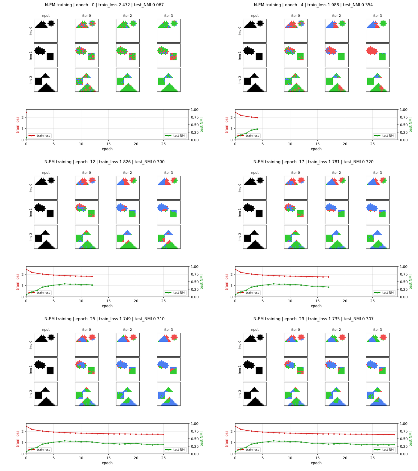
neural-em-shapes — neural-em-shapes Greff, van Steenkiste, Schmidhuber (2017), Neural EM Unsupervised perceptual grouping. K=3 slot Neural EM with manual BPTT through T=4 unrolled EM iterations. E-step softmax over pixel likelihoods, M-step tanh recurrence on bottlenecked H=24 (forces specialisation).

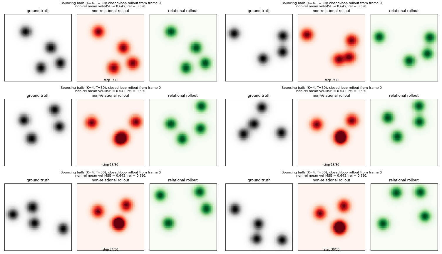
relational-nem-bouncing-balls — relational-nem-bouncing-balls van Steenkiste, Chang, Greff, Schmidhuber (2018), Relational Neural EM Bouncing balls with elastic equal-mass collisions. Oracle 4-D slot state (x, y, vx, vy). Non-relational baseline: MLP_dyn(s_k); relational: MLP_msg(s_k, s_j) to mean aggregation to MLP_dyn(s_k, agg_k). Relational wins K=3,4,5;

2018-2025, World models, fast-weight Transformers, systematic generalization

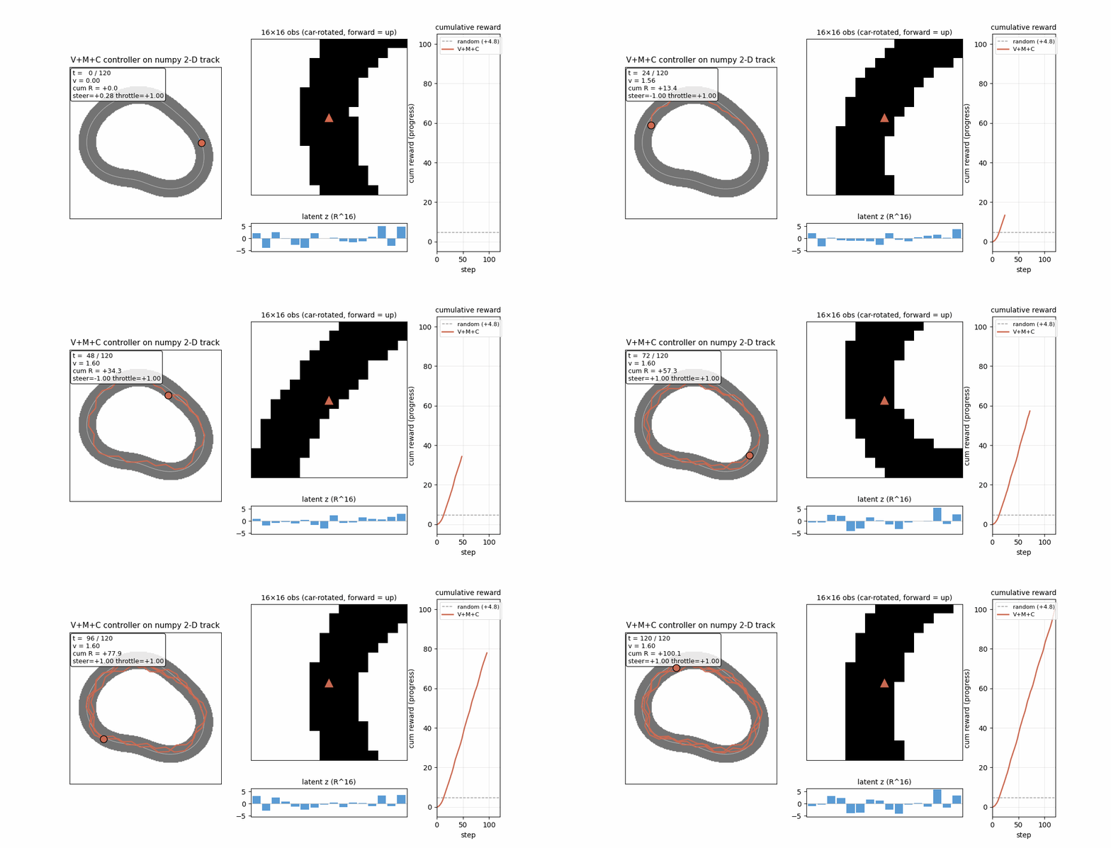
world-models-carracing — world-models-carracing Ha & Schmidhuber (2018), Recurrent World Models Numpy 2-D top-down racing track substitute for CarRacing-v0. Centerline = closed loop generated from low-frequency sinusoids; agent observes a 16×16 patch of mask, rotated to car frame.

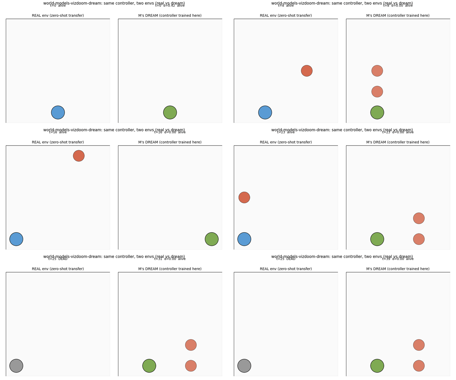
world-models-vizdoom-dream — world-models-vizdoom-dream Ha & Schmidhuber (2018), Recurrent World Models Numpy 5×5 gridworld dodging-fireballs analog of DoomTakeCover. The paper's "DoomRNN dream" experiment: controller C is trained ENTIRELY inside M's rollouts (no real-env interaction during training), then transferred zero-shot to the real env.

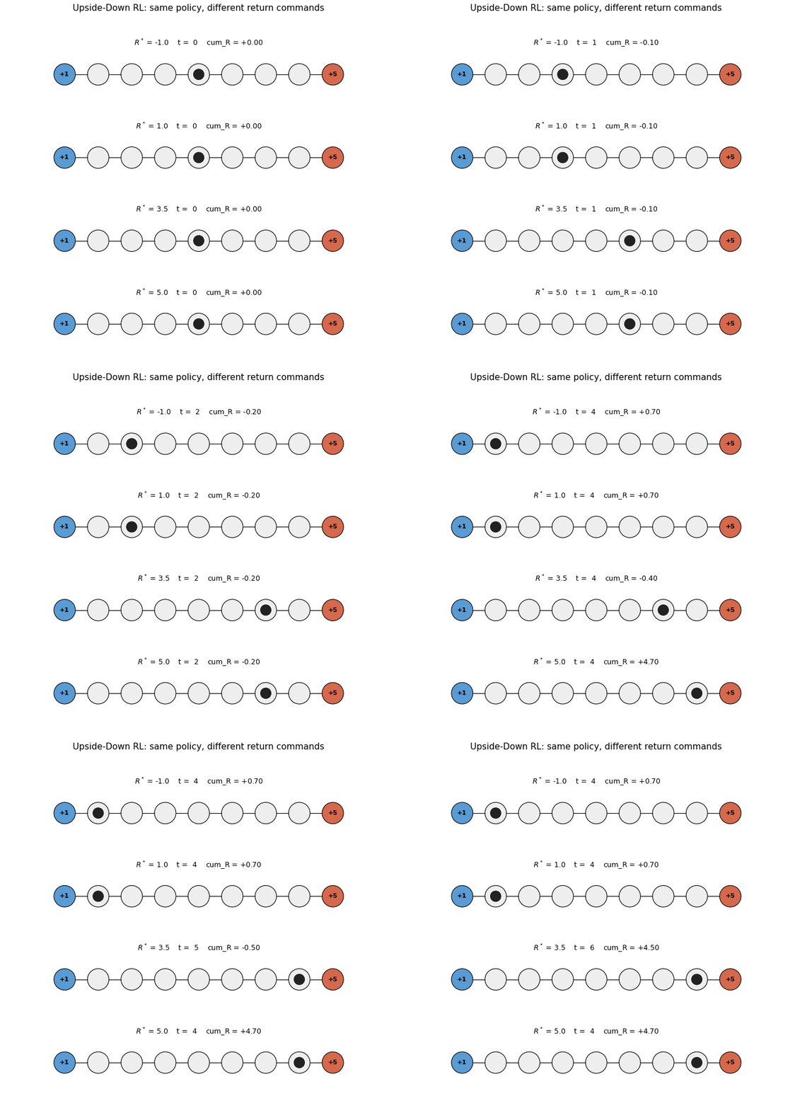
upside-down-rl — upside-down-rl Schmidhuber et al. (2019), Reinforcement Learning Upside Down Standard RL fits a value function or policy gradient. UDRL inverts: the policy is a supervised mapping from (state, desired_return, time_horizon) to action. Numpy 9-state chain MDP per SPEC's RL-stub rule (paper used LunarLanderSparse).

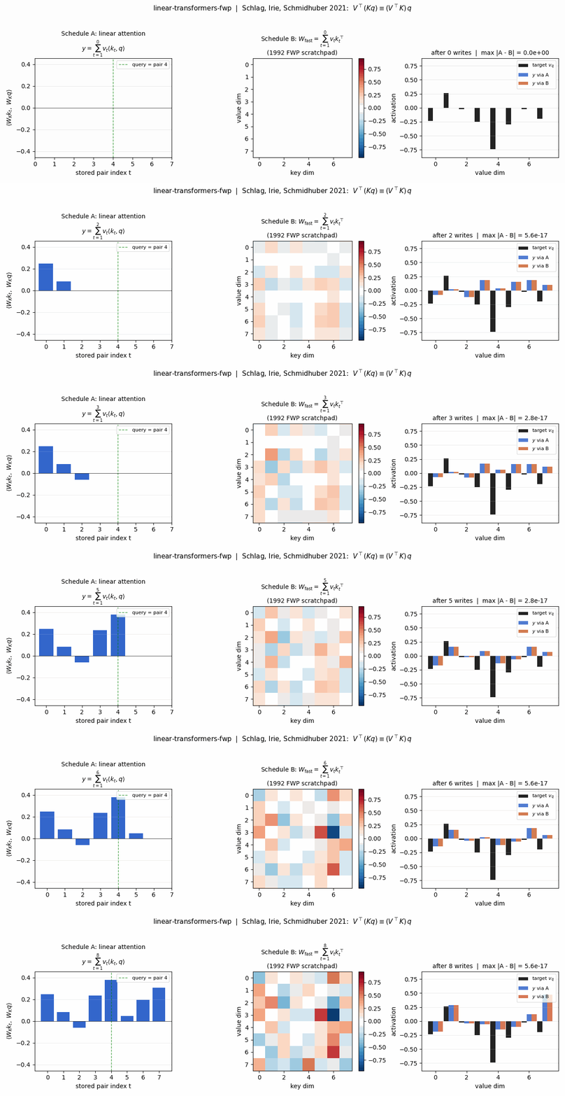
linear-transformers-fwp — linear-transformers-fwp Schlag, Irie, Schmidhuber (2021), Linear Transformers ARE Fast Weight Programmers The cleanest result of the catalog: linear self-attention V^T(Kq) and the 1992 fast-weight programmer (V^T K)q compute the same numpy expression. Equivalence verified to 2.22e-16 (1 ulp at float64) on every input tested.

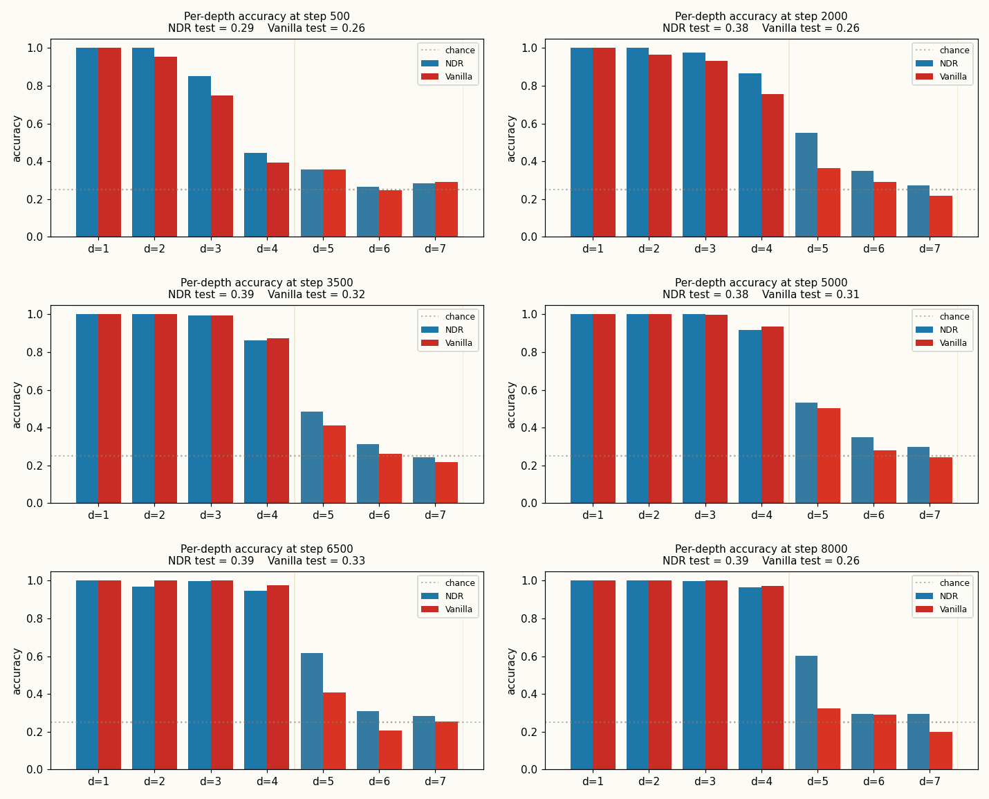
neural-data-router — neural-data-router Csordás, Irie, Schmidhuber (2022), The Neural Data Router Compositional table lookup: 4 values × 4 functions × depth-d expressions. NDR adds two switches to a Transformer: geometric attention (per-query distance-ordered scan, "stop at first match") + per-position copy gate.