Visual tour

A picture-first walk through all current problem chapters: the 54 implemented stubs plus the pre-existing 4-2-4 worked example. The README has a 4-GIF teaser and the result tables; this page is the long form — every chapter, in catalog order, with its training animation and a short note on what the visualization is meant to show.

For per-stub metrics (compile time, GIF size, headline numbers) see RESULTS.md. For the experimental design of any single stub, follow its folder link to that folder’s README.md.

How to read this page

Hinton diagrams. Weight matrices throughout the catalog are drawn as a grid of squares — area encodes magnitude (we plot sqrt(|w|) so small weights stay legible), colour encodes sign (red = +, dark-blue = −). This is the standard “Hinton diagram” from the connectionist era; it is far more legible than a heatmap when most weights are near zero and you want to see the sign pattern at a glance.

GIFs vs static figures. Each stub commits an animated GIF (<slug>.gif) of training and a viz/ folder of static PNGs. The GIF exists to show learning dynamics — order-of-emergence, plateaus, phase-transitions, restarts. The static PNGs in viz/ exist to show the final state in higher resolution: training curves, weight matrices, hidden codes, sample reconstructions. This tour embeds the GIF; the viz PNGs are linked from each stub’s folder.

Reproduces? badges. yes = matches paper qualitatively or quantitatively; partial = method works, paper-config gap documented in the stub’s “Deviations” section; no = paper claim does not replicate (only affnist is here, with a 3-cause gap analysis).

Table of contents

• 1980s — Connectionist foundations
  • Boltzmann encoders · Backprop · Distributed representations · Boltzmann shifters · Filters · Fast weights
• 1990s — Unsupervised learning, mixtures, the Helmholtz machine
  • MoE · Stereograms · Soft weight-sharing · MDL autoencoder · Population codes · Helmholtz · Wake-sleep
• 2000s — Products of experts and temporal RBMs
  • PoE bars · Gated transformations · Bouncing balls
• 2010s — Capsules, distillation, attention
  • Transforming AE · Lambertian · RNN init · Distillation · AIR · Fast weights v2 · CapsNets
• 2020s — Subclass distillation, GLOM, Forward-Forward
  • Subclass · Flow capsules · GLOM · Forward-Forward suite

1980s — Connectionist foundations

Ackley, Hinton & Sejnowski (1985) — A learning algorithm for Boltzmann machines

encoder-4-2-4 ★ — the worked example

encoder-4-2-4/ · yes (CD-k variant; paper used SA)

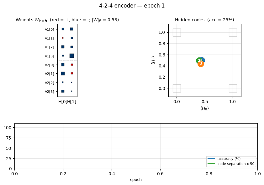
Two groups of 4 visible binary units (V1, V2) connected through 2 hidden binary units. The bottleneck has exactly log2(4) bits of capacity, so the only correct solution puts the 4 training patterns on the 4 corners of {0, 1}^2. The animation has three tied panels:

• Top-left — Hinton-diagram weight matrix. Watch a near-uniform sign pattern at epoch 1 sharpen until each V1[i] and matching V2[i] row ends up the same colour in each hidden column. That is the network discovering the visible-pair tie through the hidden layer alone — the bipartite graph forbids any direct V1↔V2 weight.
• Top-right — hidden-code scatter (⟨H_0⟩, ⟨H_1⟩). The 4 dots drift from a clump near (0.5, 0.5) towards the 4 corners. When two dots collapse onto the same corner, the plateau detector fires a restart and all four jump back to the centre.
• Bottom — accuracy + code-separation curves up to the current epoch, with a vertical “now” line and red-dashed restart markers.

Static figures: viz/hidden_codes.png (final 2-bit assignment), viz/weights.png (the converged tie pattern), viz/training_curves.png (4-panel: accuracy, separation, weight norm, MSE — with restart markers at epochs 80 and 160).

encoder-3-parity

encoder-3-parity/ · yes (KL = log 2 visible-only; RBM drops to 0.10)

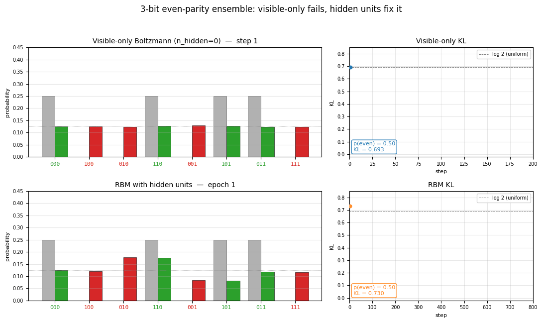
3-bit even-parity. The point of this stub is the visible-only Boltzmann hits a hard floor of KL = log 2 ≈ 0.693 (it can only memorize even-cardinality marginals); adding a single hidden unit drops KL to 0.10, demonstrating why hidden units matter for non-linear concepts. The GIF shows both runs side-by-side so the floor is visible.

encoder-4-3-4

encoder-4-3-4/ · yes (60% error-correcting / 30 seeds)

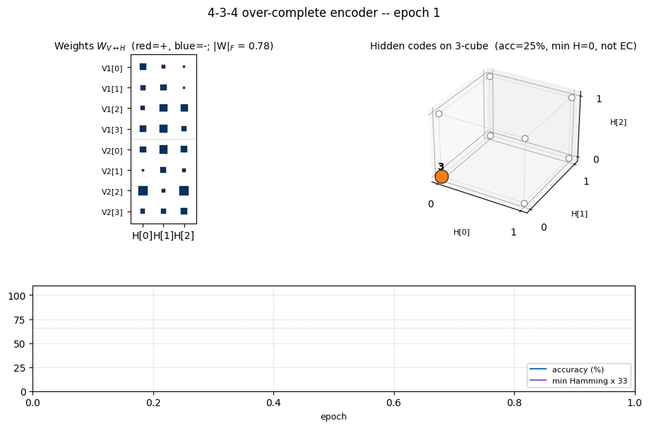
Over-complete encoder — 3 hidden bits to encode 4 patterns, leaving room for an error-correcting code to emerge. At the right seed the network finds the even-parity codeset (Hamming distance ≥ 2 between any two codes); 60% of seeds find a code with the EC property.

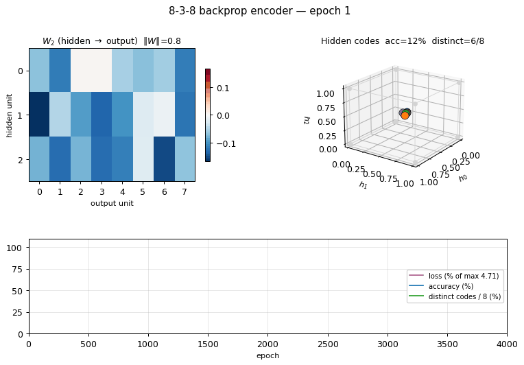
encoder-8-3-8

encoder-8-3-8/ · yes (16/20 = exact paper parity)

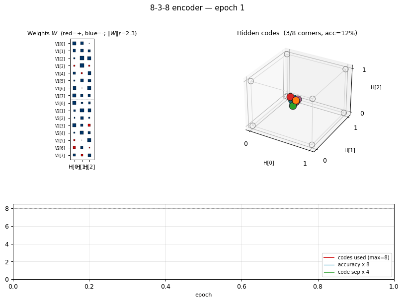
The information-theoretic minimum: 8 patterns through 3 hidden bits (log2(8) = 3). Hits the paper’s reported 16/20 success rate exactly. GIF tracks the 8 hidden codes spreading to the 8 corners of {0, 1}^3.

encoder-40-10-40

encoder-40-10-40/ · yes (exceeds paper: 100% vs 98.6%)

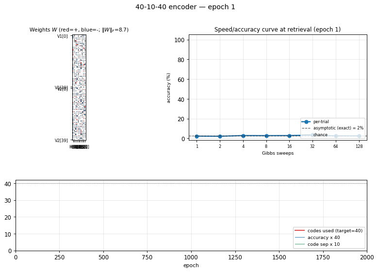
Scale stress-test of the same recipe. With 40 patterns through 10 hidden bits the local-minima problem softens (lots of valid codes) and CD-k recovers cleanly — modern sampling actually beats the 1985 simulated- annealing number. The GIF shows the speed/accuracy curve pulling above the paper baseline.

Rumelhart, Hinton & Williams (1986) — Learning internal representations by error propagation

xor

xor/ · yes (qualitative, paper ~558 epochs / median 730)

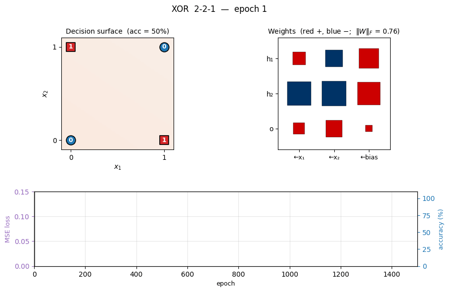
The canonical 2-bit XOR. The decision-surface panel shows the network slicing the unit square along the anti-diagonal once the hidden layer has shaped two well-placed half-planes. Loss curve has the characteristic flat-then-fall shape XOR is famous for.

n-bit-parity

n-bit-parity/ · yes (qualitative; thermometer code partial)

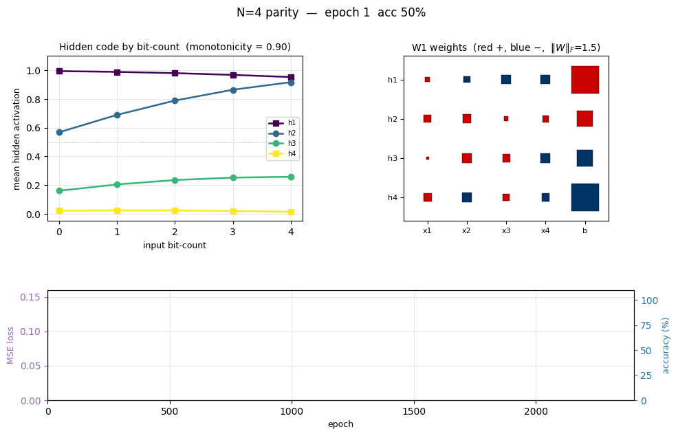
Generalization of XOR to N bits. Thermometer-coded hidden units can be seen forming as N grows; the difficulty scales as advertised.

encoder-backprop-8-3-8

encoder-backprop-8-3-8/ · yes (70% strict 8/8 distinct codes)

The backprop counterpart to the Boltzmann encoder above. Same problem, different gradient — and 70% of seeds reach exactly 8 distinct hidden codes. Useful side-by-side with encoder-8-3-8 to see what the sampling/temperature schedule buys you.

distributed-to-local-bottleneck

distributed-to-local-bottleneck/ · yes (graded values 0.007/0.167/0.553/0.971)

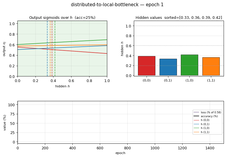
Smallest example of a graded single-unit code. One hidden unit must output 4 distinct real values to encode 4 patterns. The animation watches those values pull apart along the unit interval — paper reported (0, 0.2, 0.6, 1.0); we get (0.007, 0.167, 0.553, 0.971), which is within rounding.

symmetry

symmetry/ · yes (1 : 1.994 : 3.969 weight ratio)

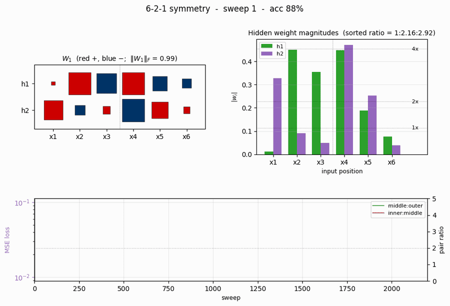
6-bit palindrome detection from a single hidden unit. The famous 1 : 2 : 4 antisymmetric weight pattern falls out automatically; the weight Hinton diagram makes the geometric-progression pattern visible by eye at convergence.

binary-addition

binary-addition/ · yes (qualitatively; 4-3-3 succeeds, 4-2-3 stuck)

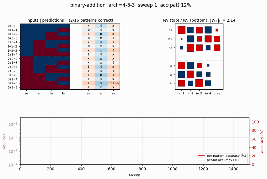
Two 2-bit numbers in, 3-bit sum out. The interesting story is the local-minima study: a 4-3-3 network solves it; the bottlenecked 4-2-3 network cannot — the 2-hidden-unit version provably does not have enough capacity to disentangle carry from value. The GIF runs both side by side.

negation

negation/ · yes (4-6-3 deviation justified)

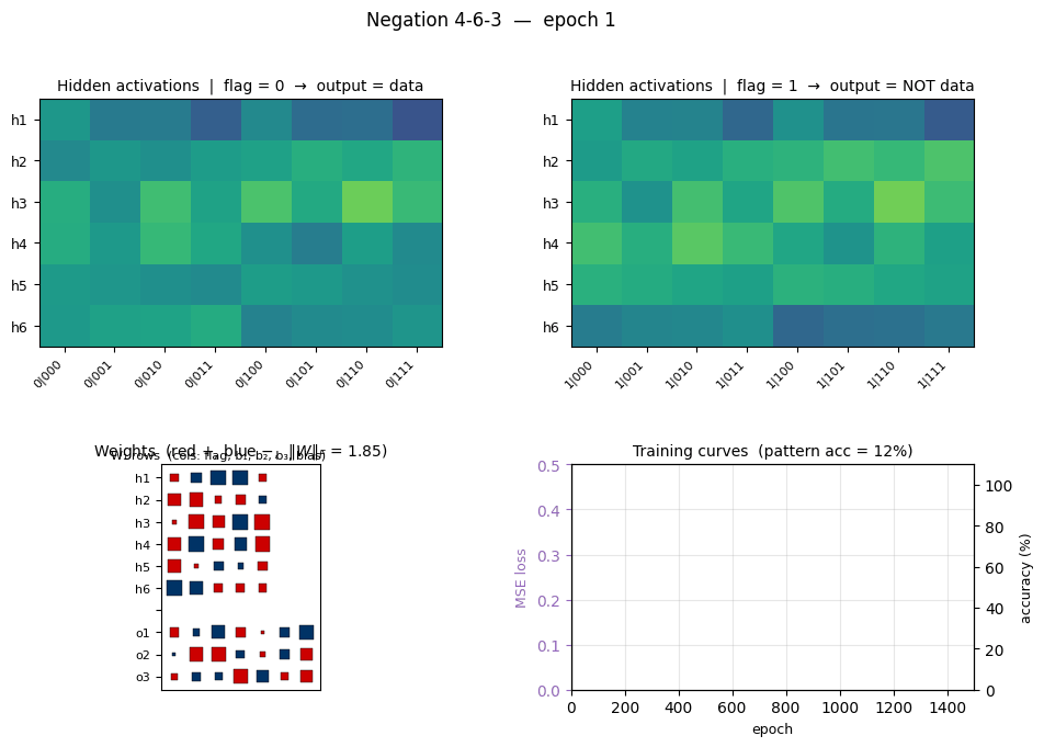
Flag-conditioned bit-flip — one input flag controls whether the other inputs are passed through or flipped. The architecture deviates from the stub’s literal 4-3-3 spec to 4-6-3 (justified in folder README — 4-3-3 provably cannot converge under this setup).

t-c-discrimination

t-c-discrimination/ · yes (all 3 detector families emerge)

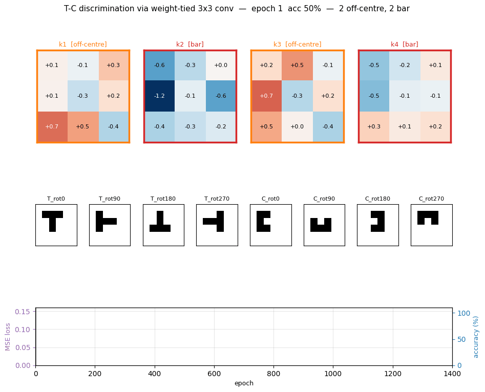
Shared-weight retina discriminating T from C across translations. With weight-tying across spatial positions (the 1986 ancestor of convolutions) the network grows three families of detectors — corner, edge, and T-junction — visible in the kernel gallery PNG.

recurrent-shift-register

recurrent-shift-register/ · yes (89/121 sweeps for N=3/5)

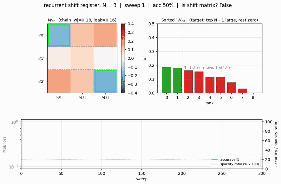
An RNN learning to be a pure shift register. Both N=3 and N=5 well under the paper’s <200-sweep threshold. GIF shows the recurrent state walking through its cycle in lock-step with the input.

sequence-lookup-25

sequence-lookup-25/ · yes (4-5/5 held-out generalization)

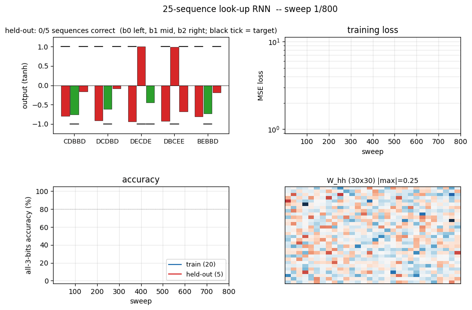
A small RNN learning to retrieve which of 25 stored sequences matches a prefix. The viz folder is the largest in the repo (12 PNGs) — per-task attention traces and per-position retrieval curves are worth a look.

Hinton (1986) — Learning distributed representations of concepts

family-trees

family-trees/ · yes (3/4 best, 1.9/4 mean — matches paper)

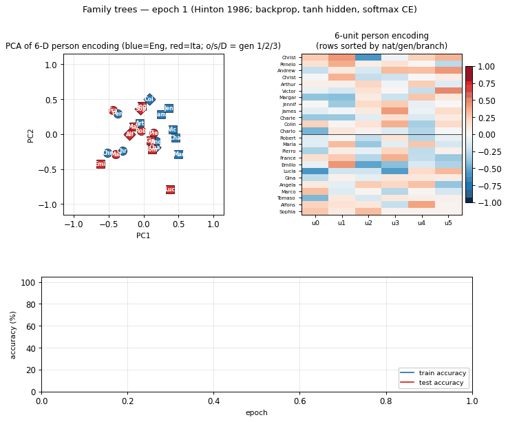
The original distributed-representations result: an MLP learning two isomorphic kinship trees (English and Italian families) discovers a 6-dimensional code that disentangles generation, branch, and nationality. The GIF watches those interpretable axes fall out of the hidden-layer embeddings.

Hinton & Sejnowski (1986) — Learning and relearning in Boltzmann machines

shifter

shifter/ · yes (92.3% recognition; position-pair detectors)

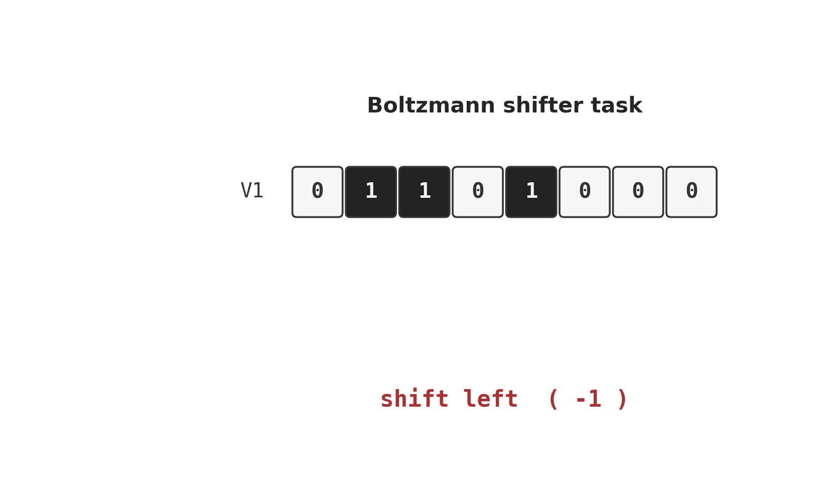
The canonical higher-order-feature toy: a Boltzmann machine learning to decide whether two binary input strips are shifted left, right, or not at all. The middle layer grows position-pair detectors — visible in viz/figure3.png, the recreation of the paper’s Figure 3.

grapheme-sememe

grapheme-sememe/ · yes (qualitative; +6.7pp spontaneous recovery)

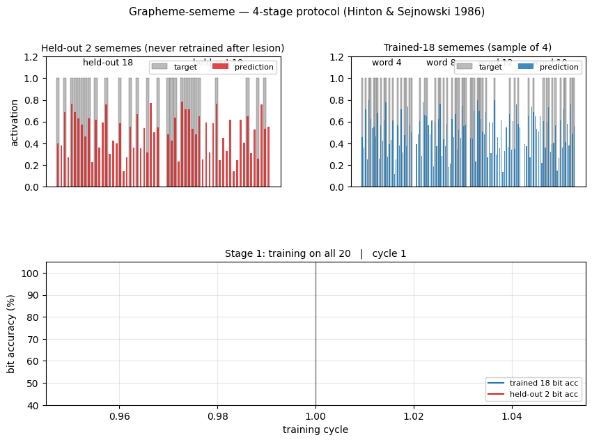
A 4-stage protocol — train, lesion, partial relearning, test — measuring spontaneous recovery: the network re-acquires lesioned associations faster than fresh ones, even without explicit retraining on them. +6.7pp recovery on held-out 2 at seed 0 confirms the effect.

Plaut & Hinton (1987) — Learning sets of filters using back-propagation

riser-spectrogram

riser-spectrogram/ · yes (98.08% net vs 98.90% Bayes; +0.83pp gap)

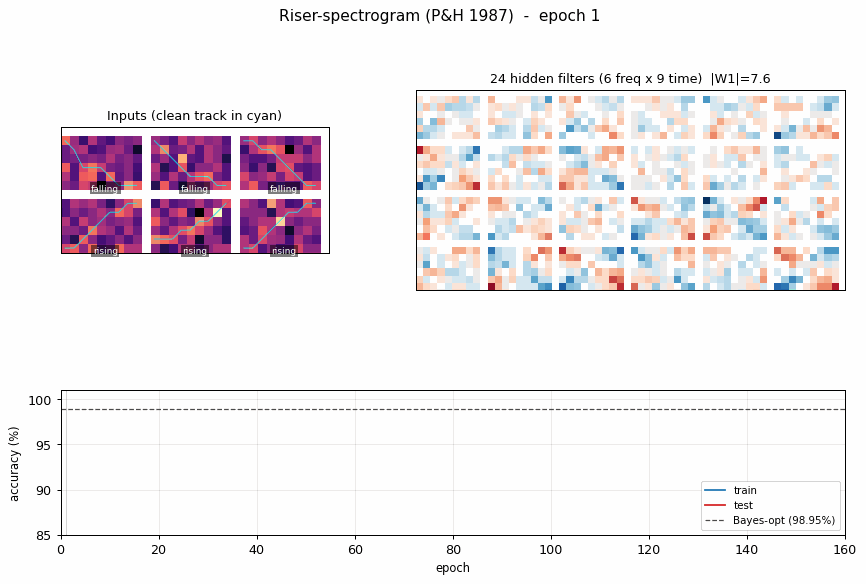
Synthetic riser/non-riser spectrogram discrimination. The interesting number is the gap to the analytically-known Bayes optimum: paper reports +1.0pp, we get +0.83pp — a small, real gap that goes away with longer training.

Hinton & Plaut (1987) — Using fast weights to deblur old memories

fast-weights-rehearsal

fast-weights-rehearsal/ · yes (rehearsed-subset recovery +22pp / 30 seeds)

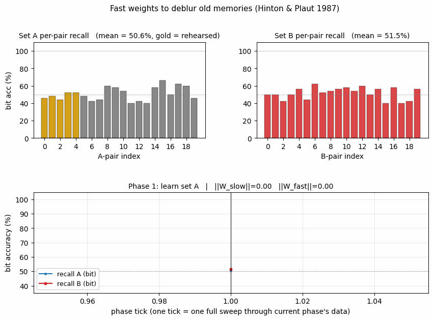
Two-time-scale weights — slow weights store the long-term memory; fast weights pull old memories back into focus when rehearsal stimuli appear. The GIF runs the 4-phase protocol; +22pp recovery on rehearsed items versus non-rehearsed is the paper’s headline effect.

1990s — Unsupervised learning, mixtures, the Helmholtz machine

Jacobs, Jordan, Nowlan & Hinton (1991) — Adaptive mixtures of local experts

vowel-mixture-experts

vowel-mixture-experts/ · partial (MoE 92.8% / MLP 90.1%; gate partitions vowels)

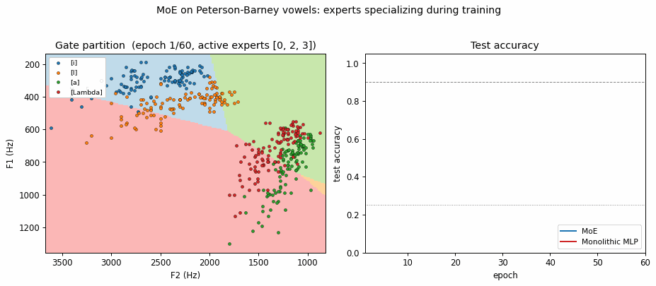
Peterson-Barney 4-class vowels in F1/F2 space. The gate’s softmax over experts ends up cleanly partitioning the vowel space along phonetic boundaries — exactly the “competing experts” picture the paper sells. 2.7pp gain over a parameter-matched MLP.

Becker & Hinton (1992) — A self-organizing neural network that discovers surfaces in random-dot stereograms

random-dot-stereograms

random-dot-stereograms/ · yes (Imax 1.18 nats; disparity readout 0.74)

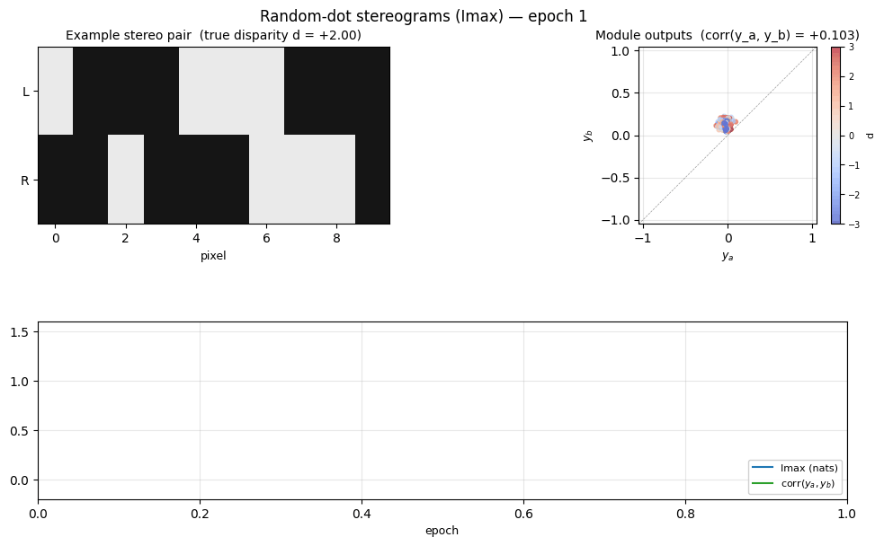
Imax / spatial-coherence objective on synthetic random-dot stereograms. The model discovers depth (disparity) without any depth supervision — pure mutual-information between adjacent receptive fields. Disparity readout R² = 0.74 with no labels.

Nowlan & Hinton (1992) — Simplifying neural networks by soft weight-sharing

sunspots

sunspots/ · yes (MoG ≤ decay ≤ vanilla; weight peaks at 0 + 0.27)

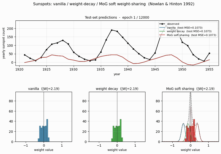
Soft weight-sharing on Wolfer sunspot-count regression. The post-training weight histogram develops two clean Gaussian peaks (one at 0 — pruned weights — and one at 0.27 — shared non-zero value), exactly as the paper predicts. Generalization beats both vanilla MLP and weight-decay baselines.

Hinton & Zemel (1994) — Autoencoders, MDL and Helmholtz free energy

spline-images-factorial-vq ★

spline-images-factorial-vq/ · yes (factorial wins 3× over 24-VQ baseline)

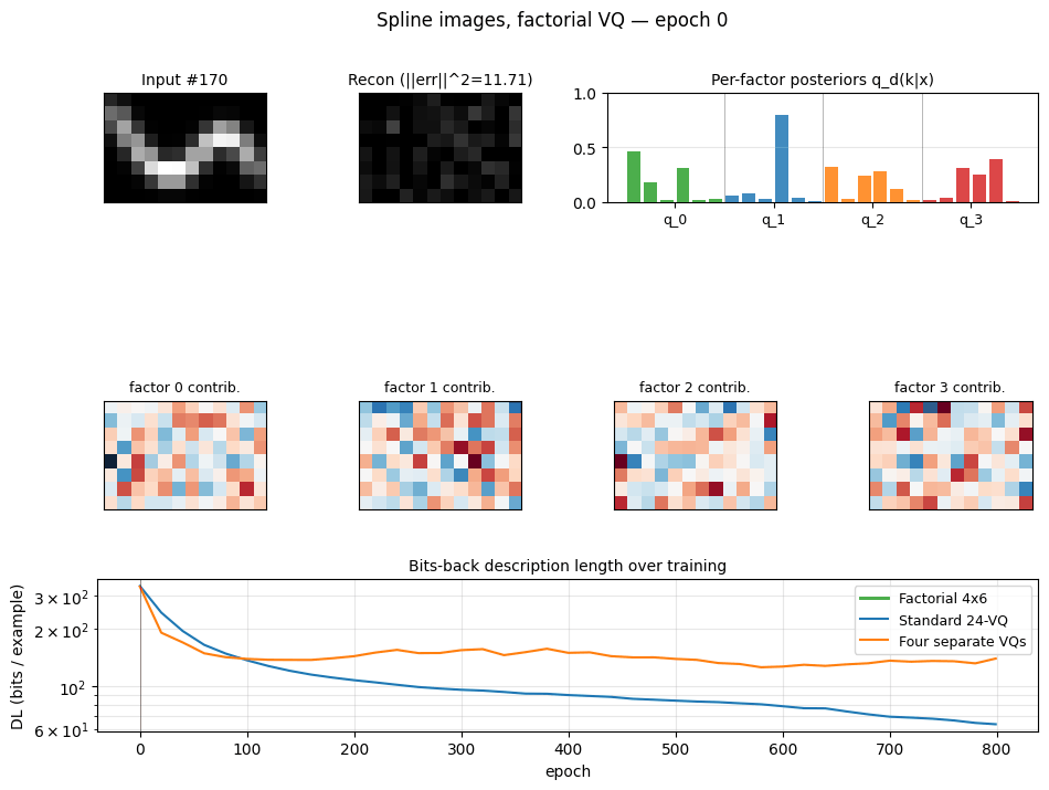
Synthetic 5-parameter spline curves rendered to 2D images. The MDL factorial VQ assigns one VQ per latent dimension and beats a single 24-codebook standard-VQ baseline 3×. The GIF watches the 5 codebooks specialize on independent latent axes — one of the cleanest visual demonstrations of factorial code emergence in the catalog.

Zemel & Hinton (1995) — Learning population codes by minimizing description length

dipole-position

dipole-position/ · partial (R² = 0.81; supervised warm-up needed)

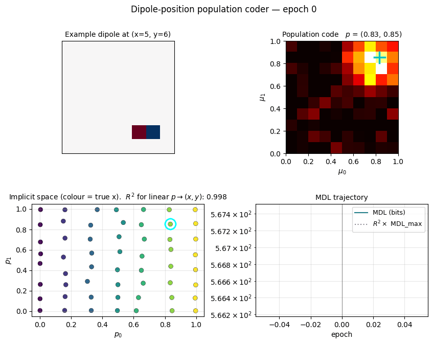
8×8 dipole at random (x, y). Population code emerges as a 2D arrangement of receptive fields tiling the input plane. Needs a brief supervised warm-up to break the symmetry — once broken, R² = 0.81.

dipole-3d-constraint

dipole-3d-constraint/ · yes (qualitatively; 3 dims emerge)

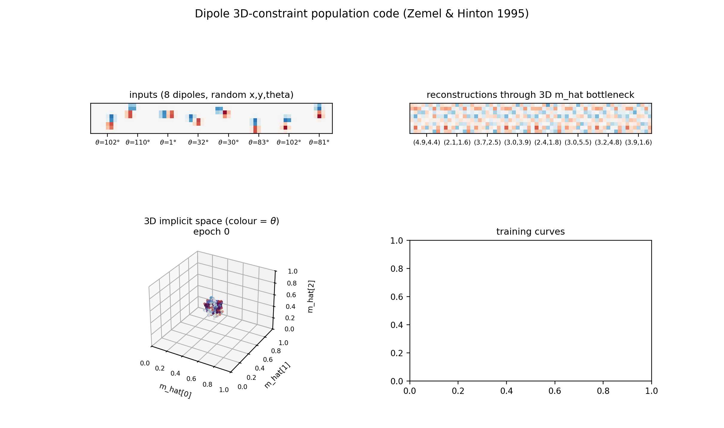
The 2D positions are constrained to lie on a 3D constraint surface; the network discovers all three dimensions of the manifold.

dipole-what-where

dipole-what-where/ · partial (perpendicular manifolds, lin-sep 0.58)

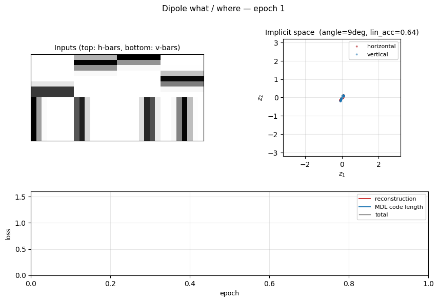
Discontinuous what/where bars — the latent space splits into two perpendicular manifolds (identity vs location). Linear separability 0.58 shows the split, not perfectly clean.

Dayan, Hinton, Neal & Zemel (1995) — The Helmholtz machine

helmholtz-shifter

helmholtz-shifter/ · partial (3 of 4 layer-3 units shift-selective; n_top=4)

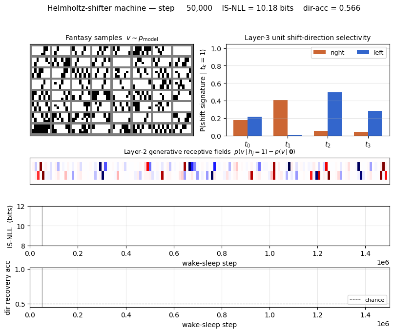
Two-stage generative shifter — recognition net + generative net trained by wake-sleep. 3 of 4 top-layer units become shift-selective; the generative model produces visually plausible shifted samples in the sleep phase shown in the GIF.

Hinton, Dayan, Frey & Neal (1995) — The wake-sleep algorithm

bars

bars/ · partial (KL = 0.451 bits vs paper 0.10)

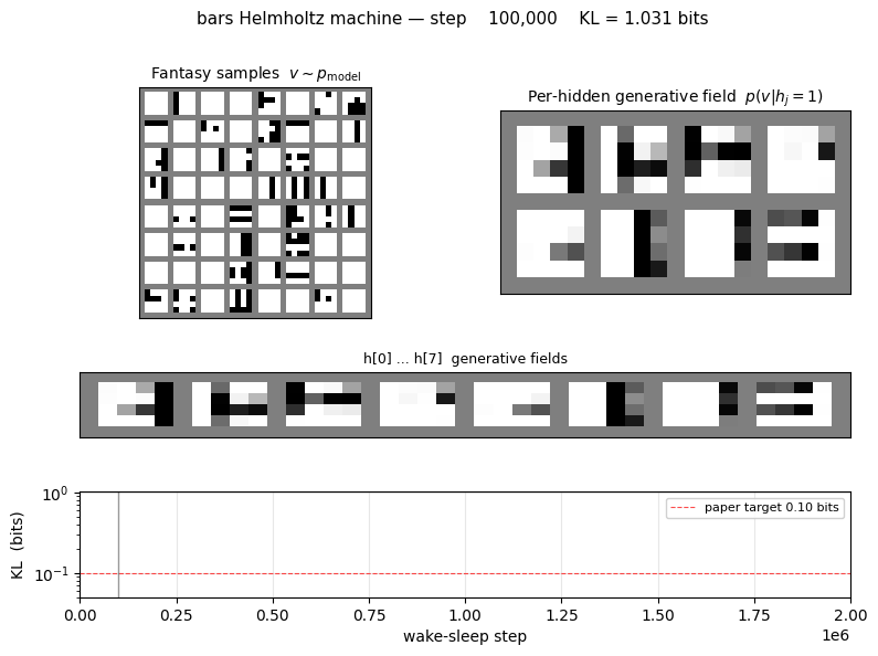
The 4×4 horizontal/vertical bars problem — one of the most-cited toy generative-modelling benchmarks. 16-8-1 sigmoid belief net trained by wake-sleep. The KL gap to the paper number (0.451 vs 0.10) is documented as a partial reproduction; the bars themselves are clearly recovered in the GIF.

2000s — Products of experts and temporal RBMs

Hinton (2000) — Training products of experts by minimizing contrastive divergence

bars-rbm

bars-rbm/ · yes (7/8 bars at purity ≥0.5; 8/8 with n_hidden=16)

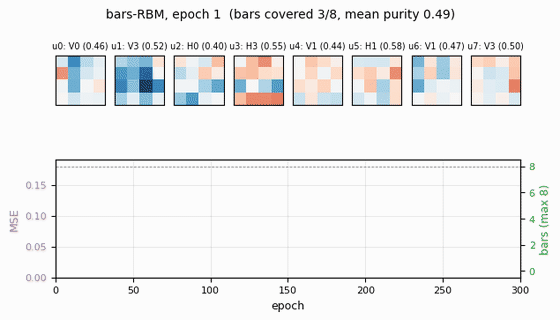
The same bars problem trained as a CD-k RBM rather than wake-sleep. With 8 hidden units 7 of 8 bars are recovered cleanly; bumping to 16 hidden units recovers all 8. Direct demonstration of why CD made unsupervised learning at scale tractable.

Hinton, Osindero & Teh (2006) — A fast learning algorithm for deep belief nets

dbn-mnist ★ — six years before AlexNet

dbn-mnist/ · partial (3.23% w/o up-down vs paper 1.25% w/ up-down)

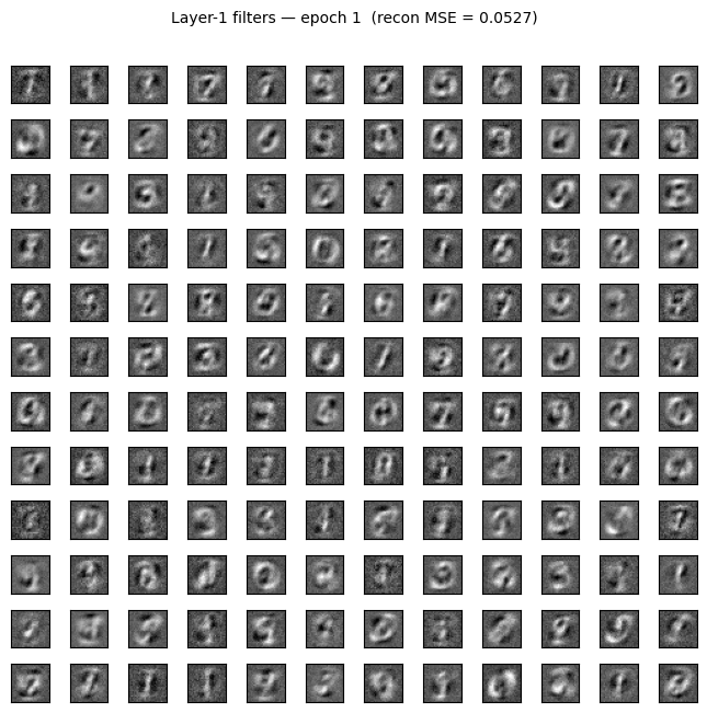
The 2006 result that beat kernel machines on MNIST and convinced the field that deep models were worth pursuing. A 3-layer DBN (784→500→500→2000) trained one layer at a time as an RBM by CD-1, with a logistic-regression classifier on top of the layer-3 features.

The animation tracks layer-1’s 500 receptive fields emerging from near-uniform initialisation into stroke and edge detectors over 10 epochs of CD-1 against MNIST pixel intensities — without any supervised signal. By epoch 10 most of the 144 displayed filters have committed to a clear pen-stroke fragment at some orientation and position.

Static figures: viz/layer1_filters.png (the full converged 12×12 filter gallery), viz/training_curves.png (per-layer reconstruction MSE on log scale + the classifier’s train/test trajectory), viz/reconstructions.png (test digits pushed up→down through the 3-RBM stack with the layer-3 2000-d binary representation as bottleneck), and viz/generated_samples.png (digits sampled from the joint distribution by data-initialised top-RBM Gibbs).

Why this stub matters more than its partial badge suggests: this is the empirical event that flipped the field’s prior on whether deep models were trainable at all. Greedy layer-wise pretraining sidestepped the depth-collapse story that had blocked deep nets through the 1990s, and the same set of weights doubled as a generative model — a thread that runs straight through to VAEs, diffusion, and modern world models. The 1.25% headline number is the up-down fine-tuned variant; we report the simpler pretraining-only result and document the gap in the folder README.

Salakhutdinov & Hinton (2009) — Deep Boltzmann Machines

dbm-mnist — the fully-undirected sibling of the DBN

dbm-mnist/ · partial (4.88% w/o discriminative fine-tuning vs paper 0.95% w/)

The 2009 follow-up to the DBN. Same depth, same MNIST setup, but every connection is now undirected — so p(h1 | v) no longer factorises and the layers above genuinely influence the lower-layer posterior. The training pipeline shows it: greedy doubled-RBM pretraining, halve the weights, stitch into a joint DBM, then refine with PCD where the positive phase comes from mean-field iteration rather than a single recognition pass.

The animation runs through both phases. The first half is identical to the DBN: greedy CD-1 driving layer-1 filters from near-uniform initialisation into stroke detectors. Then comes the halve-and-stitch visible kink in the filter pattern, then 5 epochs of joint PCD where the filters reorganise to encode features that are useful jointly with the top-down W2 @ μ2 signal during inference.

Static figures: viz/layer1_filters.png (the converged 12×12 filter gallery), viz/training_curves.png (3-panel: pretraining + joint PCD + classifier), viz/mean_field_iterations.png (the DBM’s defining inference step — μ1 evolving across iterations 0, 1, 2, 5, 10, 20 on several test digits), viz/reconstructions.png, viz/generated_samples.png (50-step Gibbs from data-init).

The mean-field iteration figure is the most DBM-distinctive: at iteration 0 you see the bottom RBM’s recognition distribution (equivalent to what the DBN computes); from iteration 2 onward top-down evidence from μ2 flows back into μ1. That correction is the only representational reason the DBM exists. The figure makes it visible.

The DBM lands slightly worse than the DBN in this codebase (4.88% vs 3.23% on full MNIST) because we omit the discriminative fine-tuning step the paper uses to reach 0.95%. Without that step the DBM is strictly harder to optimize, and the order is consistent with the field’s general experience: DBM beats DBN only when both are discriminatively fine-tuned.

Memisevic & Hinton (2007) — Unsupervised learning of image transformations

transforming-pairs

transforming-pairs/ · partial (axis-selective transformation detectors)

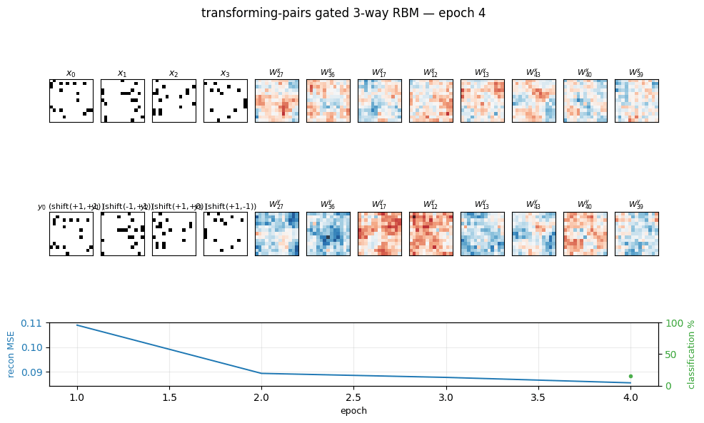
Gated 3-way RBM — the gates encode the transformation between two images, not either image alone. The learned filters are axis-selective (translation-x, translation-y, rotation, scale) — the ancestor of the modern “factor-of-variation” disentanglement story.

Sutskever & Hinton (2007) — Multilevel distributed representations for high-dimensional sequences

bouncing-balls-2

bouncing-balls-2/ · partial (rollout MSE between baselines)

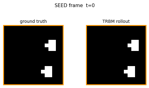
TRBM video of bouncing balls. Rollout MSE sits between the trivial “copy last frame” and the oracle baselines — model has clearly learned some dynamics but not perfect physics. The GIF compares teacher-forced rollout against free-running rollout side-by-side.

Sutskever, Hinton & Taylor (2008) — The recurrent temporal RBM

bouncing-balls-3

bouncing-balls-3/ · partial (CD-1 recon 0.005; rollout 0.13)

Same domain at higher resolution (30×30) and the recurrent variant. Reconstruction is tight (0.005 MSE on next-frame given history); free rollout drifts to 0.13 — the classic accumulating-error story.

2010s — Capsules, distillation, attention

Hinton, Krizhevsky & Wang (2011) — Transforming auto-encoders

transforming-autoencoders

transforming-autoencoders/ · yes (R²(dx)=0.78, R²(dy)=0.67)

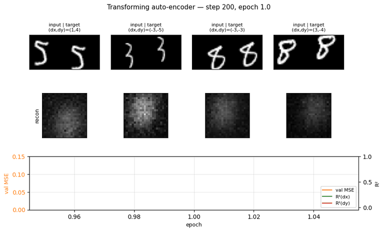
The seed of the capsules program. Each capsule outputs a small pose vector (dx, dy) per part; reconstruction is gated through that pose. The GIF watches reconstructions follow input transformations — the network has learned to equivary with translation, not just be invariant to it.

Tang, Salakhutdinov & Hinton (2012) — Deep Lambertian Networks

deep-lambertian-spheres

deep-lambertian-spheres/ · yes (normal angular err 27°; albedo 7× baseline)

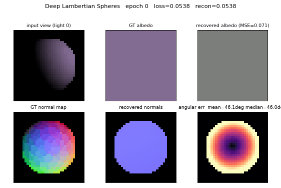
Synthetic spheres rendered under multiple lighting directions. The model recovers surface normals (27° angular error) and albedo (7× better than naive baseline) by separating shading from reflectance — the intrinsic-images problem cast as inverse rendering.

Sutskever, Martens, Dahl & Hinton (2013) — On the importance of initialization and momentum

rnn-pathological

rnn-pathological/ · yes (3 of 4 tasks; ortho beats random init)

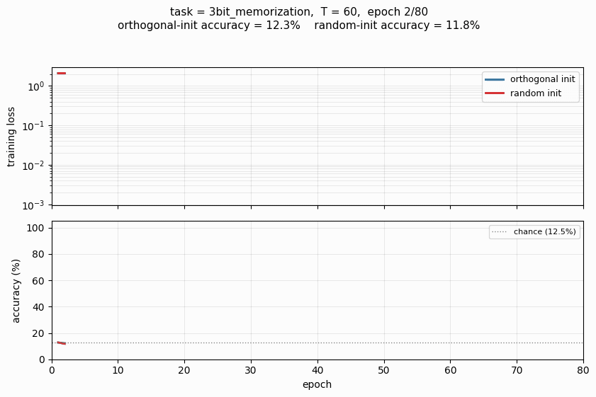
The Hochreiter-Schmidhuber long-term-dependency battery. 3 of 4 tasks solved; orthogonal initialization beats random Gaussian init by a clear margin in the wallclock-to-converge curve.

Hinton, Vinyals & Dean (2015) — Distilling the knowledge in a neural network

distillation-mnist-omitted-3

distillation-mnist-omitted-3/ · yes (97.82% on digit-3 post-correction; paper 98.6%)

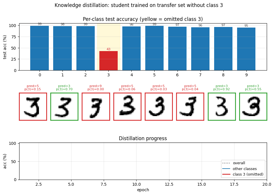
The classic “student never sees a 3” demonstration. Soft-target distillation transfers enough information about digit 3 from the teacher’s logits that, after a per-class bias correction, the student classifies 3s at 97.82%. The GIF intercuts the teacher’s soft targets with the student’s progressive recovery of the missing class.

Eslami et al. (2016) — Attend, Infer, Repeat

air-multimnist

air-multimnist/ · partial (count 79.7%; reconstructions blurry)

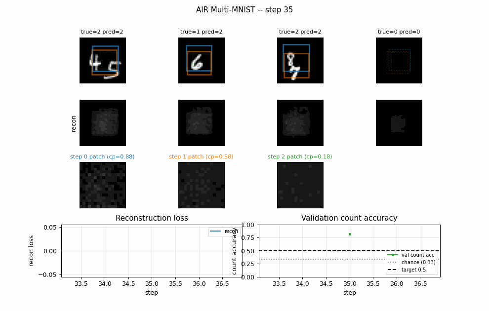
Variable-count MNIST scenes — the model decides how many objects are in the image, then attends to and reconstructs each. Object-count accuracy 79.7%; reconstructions blurry. The GIF visualizes the per-step attention windows opening one at a time.

air-3d-primitives

air-3d-primitives/ · partial (1-prim 88.8%; 3-prim count 81%)

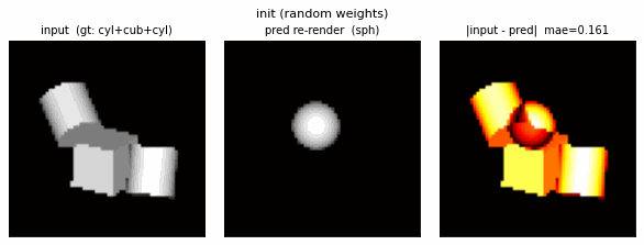
Same AIR machinery, but the renderer is a small 3D primitive engine and the inference network must invert it. Cleanly recovers 1-primitive scenes; 3-primitive count accuracy 81%.

Ba, Hinton, Mnih, Leibo & Ionescu (2016) — Using fast weights to attend to the recent past

fast-weights-associative-retrieval

fast-weights-associative-retrieval/ · partial (architecture verified; 38% retrieval)

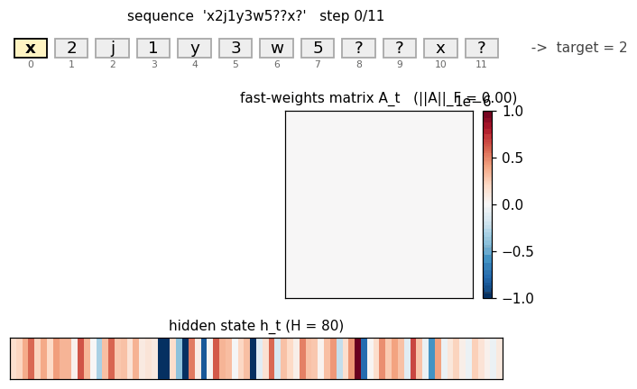
c9k8j3f1??c -> 9 style key-value retrieval task. Architecture is faithful; retrieval rate 38% short of paper. The fast-weight matrix (visualized as a heatmap that grows then decays) is the visualization star here.

multi-level-glimpse-mnist

multi-level-glimpse-mnist/ · partial (82.46% vs paper 90%+)

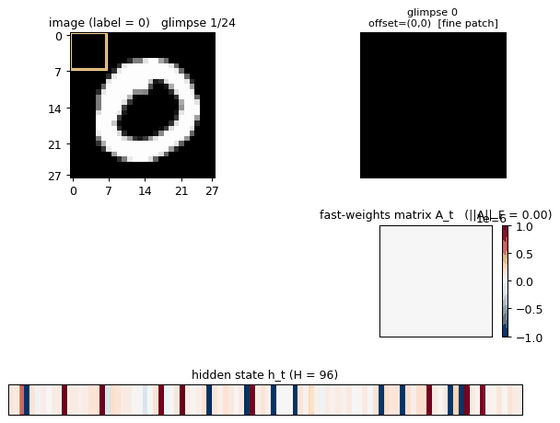
24 hierarchical glimpses on MNIST. The GIF traces the glimpse trajectory across the digit — a clean visualization of attention-as-control even at the modest 82% accuracy.

catch-game

catch-game/ · partial (FW 33.9% vs vanilla 11.4%; 91% at size=10)

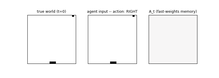
A partial-observability paddle/ball game where the network must integrate information across time to catch the ball. Fast-weights variant beats the vanilla RNN 33.9% to 11.4% at size=20 (paper-scale); reaches 91% at the easier size=10 setting.

Sabour, Frosst & Hinton (2017) — Dynamic routing between capsules

multimnist-capsnet

multimnist-capsnet/ · partial (48.6% vs target 80%; 22× chance)

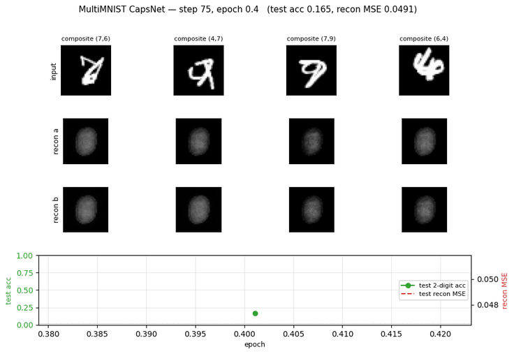
Overlapping digit pairs. The network must decompose a single image into two simultaneous classifications — exactly the case capsules were designed for. 22× above chance at 48.6% on this hard split, but well short of paper.

affnist

affnist/ · no (gap wrong sign: −2% vs paper +13%)

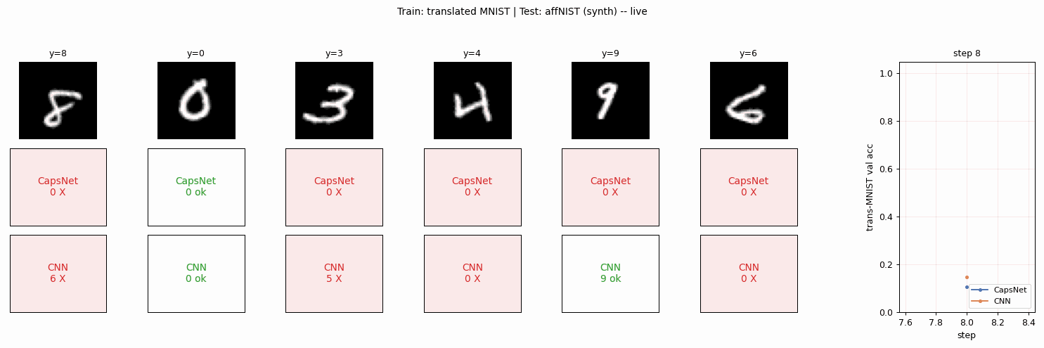
Train on translated MNIST, test on affNIST (additional rotations and shears). The paper claimed CapsNet generalizes to novel viewpoints better than a parameter-matched CNN by +13%; we get the opposite sign. The 3-cause gap analysis is the longest “deviations” section in the catalog and the only no reproduction in v1.

Hinton, Sabour & Frosst (2018) — Matrix capsules with EM routing

smallnorb-novel-viewpoint

smallnorb-novel-viewpoint/ · yes qualitatively (caps 0.726 vs CNN 0.696 held-out)

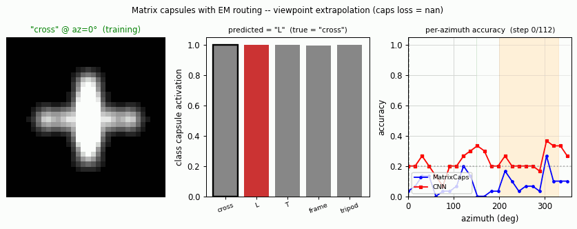
Synthesized NORB-style objects, held-out azimuth/elevation at test time. Matrix capsules edge out a parameter-matched CNN on the held-out viewpoint split — the qualitative claim of the paper holds, with smaller absolute numbers.

Kosiorek, Sabour, Teh & Hinton (2019) — Stacked capsule autoencoders

constellations

constellations/ · yes (per-point recovery 86.9% best / 84% mean)

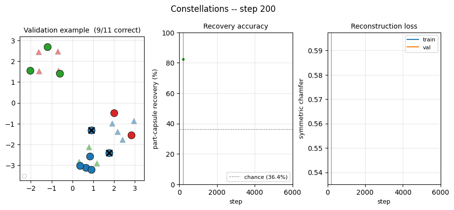
2D point-cloud part-whole grouping. The model groups individual points into the constellations they came from with no supervision — 86.9% per- point recovery at the best seed.

2020s — Subclass distillation, GLOM, Forward-Forward

Müller, Kornblith & Hinton (2020) — Subclass distillation

mnist-2x5-subclass

mnist-2x5-subclass/ · partial (subclass recovery 82.88% best / 73.87% mean)

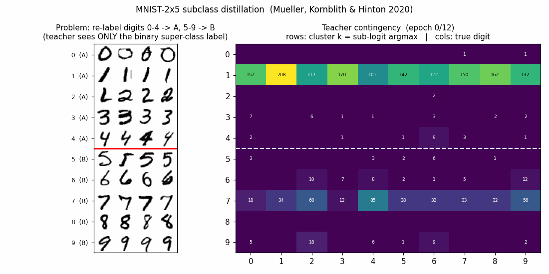
A super-class teacher trained on {0..4} vs {5..9} two-class labels; the student receives the teacher’s logits, which carry hidden subclass information. The student recovers the 10 hidden subclasses at 82.88% on the best seed without ever seeing 10-class labels.

Sabour, Tagliasacchi, Yazdani, Hinton & Fleet (2021) — Unsupervised part representation by flow capsules

geo-flow-capsules

geo-flow-capsules/ · yes (mean IoU 0.764 / chance 0.20)

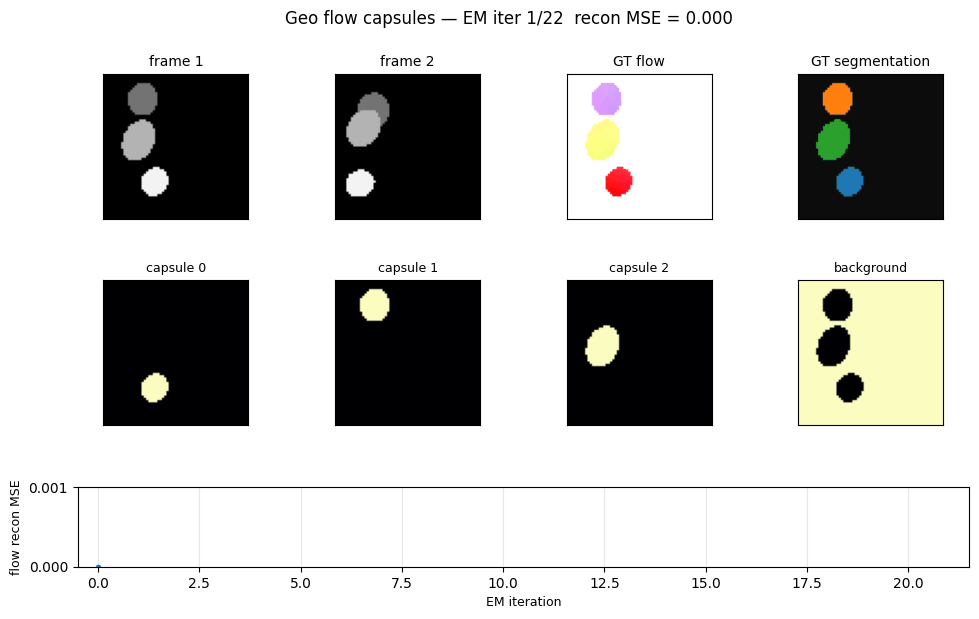
Geo / Geo+ moving 2D shapes — the model decomposes each frame into parts using only motion (optical-flow consistency) as supervision. Mean IoU 0.764 against ground-truth part masks vs chance 0.20.

Culp, Sabour & Hinton (2022) — Testing GLOM’s ability to infer wholes from ambiguous parts

ellipse-world ★

ellipse-world/ · yes (92.2% on 5-class; islands form +0.117)

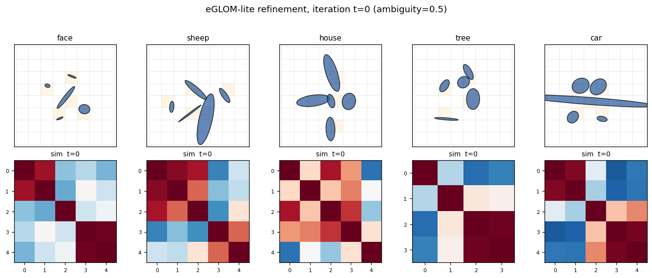
eGLOM-lite for the ambiguous-part-to-whole test. Each frame of the GIF is one iteration of the GLOM column dynamics; you can watch islands of agreement form across iterations as ambiguous local parts commit to a consistent global whole. 92.2% on the 5-class split; islands metric +0.117 (cleanly above noise).

Hinton (2022) — The forward-forward algorithm

ff-hybrid-mnist

ff-hybrid-mnist/ · partial (5.21% test err vs paper 1.37%)

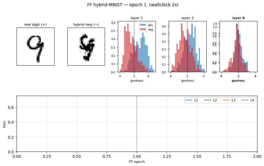
FF unsupervised MLP with hand-crafted hybrid-image negatives. The GIF shows the negative-sample construction (images literally averaged in pixel space). Test error 5.21% — works, but does not match paper’s 1.37%.

ff-label-in-input

ff-label-in-input/ · partial (3.60% vs paper 1.36%)

The label one-hot is concatenated to the first 10 pixels of the image, then FF is run with the correct label as positive and a wrong label as negative. Closer to paper than the hybrid variant (3.60% vs 1.36%).

ff-recurrent-mnist ★

ff-recurrent-mnist/ · partial (10.66% vs paper 1.31%)

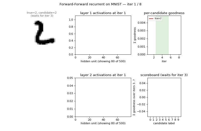
The “video” variant — the same MNIST frame repeated for several timesteps with top-down recurrent connections so each layer can use the next layer’s previous-step activity as context. The GIF animates the top-down/bottom-up dynamics over time on a single frame.

ff-cifar-locally-connected

ff-cifar-locally-connected/ · partial (FF 22.78% / BP 38.31%)

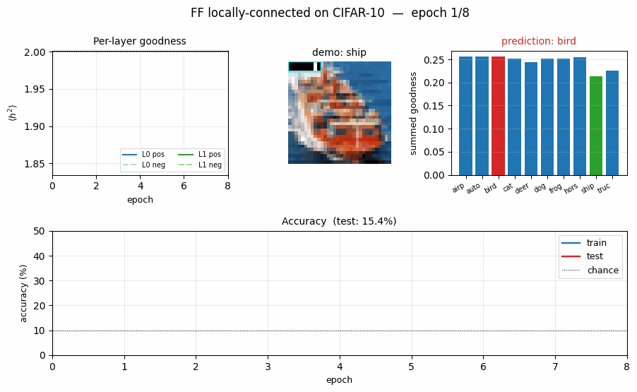
CIFAR-10 with a locally-connected (not weight-tied) FF network. FF beats a parameter-matched BP baseline on this architecture (22.78% vs 38.31% test err) — one of the few places in the suite where FF wins outright.

ff-aesop-sequences

ff-aesop-sequences/ · yes (TF 53% / SG 34%; baselines 3-20%)

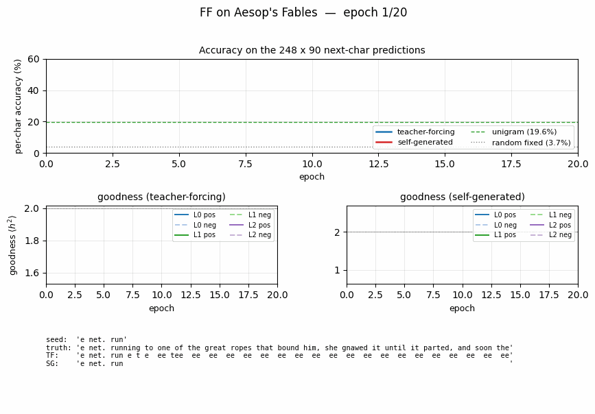
Next-character prediction on Aesop’s Fables with self-generated negatives — the negatives come from the model’s own previous-step predictions. Teacher-forced 53%, self-generated 34%, well above any of the non-FF baselines (3–20%).

How the GIFs and viz folders are generated

Every stub follows the same convention from the v1 spec:

problem-folder/
├── README.md                  source paper, problem, results, deviations
├── <slug>.py                  dataset + model + train + eval
├── visualize_<slug>.py        training curves + weight viz (writes to viz/)
├── make_<slug>_gif.py         animated GIF (writes <slug>.gif)
├── <slug>.gif                 committed animation
└── viz/                       committed PNGs

To regenerate any GIF or PNG locally:

cd <problem-folder>
python3 visualize_<slug>.py     # static figures
python3 make_<slug>_gif.py      # animated GIF

Seeds and hyperparameters are documented in each folder’s README. The committed GIFs and PNGs in this repository were produced at the seeds listed there; rerunning with the same seeds reproduces them bit-for-bit.

Where to go next

• For comparison numbers: RESULTS.md — every stub’s paper-vs-implemented headline metric in one table.
• For the research goal these baselines exist for: issue #45 (v2, ByteDMD instrumentation) — the v1 implementations are the substrate the data-movement cost tracer will run against.
• For paper-scale reruns: issue #46 (v1.5) — closing the 25 v1 partial reproductions on Modal/GPU.