Bars problem for RBM training
Source: Hinton, G. E. (2000), “Training products of experts by minimizing contrastive divergence” (Gatsby tech report; Neural Computation 14(8), 2002). The bars task itself is from Foldiak, P. (1990), “Forming sparse representations by local anti-Hebbian learning.”
Demonstrates: the canonical sanity check for RBM / contrastive-divergence training — after CD-1 training, each hidden unit specializes to a single bar.
Problem
- Visible: 16 binary pixels arranged as a 4×4 image.
- Hidden: 8 binary feature detectors (canonical setting; one per bar).
- Connectivity: bipartite RBM (visible ↔ hidden only).
- Training distribution: each image is generated by independently
activating each of 8 single-bar templates (4 horizontal rows + 4 vertical
columns) with probability
p_bar = 1/8, then taking the logical OR over activated bars to get the pixels. So each image is a superposition of bars.
The interesting property: the data has a clean latent factor structure (8 independent on/off causes), but the visible pixels are tangled by the OR mixture. Backprop on a single image cannot recover the bars, because there is no per-pixel target. The RBM gets the bars from the statistics alone: under CD-1, each hidden unit learns to fire iff one specific bar is present, because that maximizes the model’s likelihood under the bipartite factorization.
The trick is that an over-explanatory hidden code (e.g. one unit that fires for any bar) reconstructs the data poorly — the model needs distinct units for distinct causes. Sparsity in the hidden activations + the bipartite structure together make the per-bar decomposition the natural local optimum.
Files
| File | Purpose |
|---|---|
bars_rbm.py | Bars dataset + BarsRBM + cd1_step() + train() + per_unit_bar_purity() + visualize_filters(). CLI for reproducing the headline run. |
visualize_bars_rbm.py | Static PNGs: receptive fields, training curves, sample reconstructions, data examples, bar-template reference. |
make_bars_rbm_gif.py | Generates bars_rbm.gif (the animation at the top of this README). |
bars_rbm.gif | Receptive fields evolving across 300 epochs of CD-1. |
viz/ | Output PNGs from the headline seed=2 run. viz/n_hidden_16/ holds the over-complete (n_hidden=16) sibling run. |
problem.py | The original stub signatures. Re-exports from bars_rbm.py. |
Running
python3 bars_rbm.py --seed 2 --n-hidden 8 --n-epochs 300
Training time: ~1.5 s on a laptop. Final result for seed=2: 7/8 bars
recovered, mean per-unit purity 0.90, reconstruction MSE 0.016.
To regenerate visualizations:
python3 visualize_bars_rbm.py --seed 2 --n-hidden 8 --n-epochs 300
python3 make_bars_rbm_gif.py  --seed 2 --n-hidden 8 --n-epochs 300
To explore over-complete coding (more hidden units than bars):
python3 visualize_bars_rbm.py --seed 0 --n-hidden 16 --n-epochs 300 \
    --outdir viz/n_hidden_16
Results
Headline run (n_hidden = 8, seed = 2)
| Metric | Value |
|---|---|
| Bars recovered (purity ≥ 0.5) | 7 / 8 |
| Mean per-unit purity | 0.90 |
| Reconstruction MSE (one CD step) | 0.016 |
| Training time | ~1.5 s |
Convergence statistics (10 seeds, n_hidden = 8)
| Outcome | Count |
|---|---|
| ≥ 7 bars recovered | 8 / 10 |
| All 8 bars recovered | 2 / 10 |
| Mean bars / 8 | 7.0 |
So the typical outcome is “7 of 8 hidden units lock onto distinct bars; one unit duplicates a neighbour or stays partially mixed.” That is the standard CD-1-on-bars result reported in the original literature — cleaner sparsity penalties or PCD push the rate higher (see Open questions below).
Over-complete (n_hidden = 16, seed = 0)
| Metric | Value |
|---|---|
| Bars recovered | 8 / 8 |
| Mean per-unit purity | 0.94 |
| Reconstruction MSE | 0.0001 |
| Training time | ~2.8 s |
With twice the hidden units, every bar is found by at least one unit. Some units duplicate (two units detecting the same bar), some learn slightly shifted/rotated mixtures — but no bar is missed.
Hyperparameters used
| Param | Value |
|---|---|
n_train (samples) | 2000 |
batch_size | 20 |
lr | 0.10 |
momentum | 0.5 |
weight_decay (L2) | 1e-4 |
sparsity_cost | 0.1 |
sparsity_target | 1 / n_hidden |
init_scale (W) | 0.01 |
b_v init | logit(data_mean) |
b_h init | logit(sparsity_target) |
p_bar (per-bar activation prob) | 0.125 |
n_epochs | 300 |
Visualizations
Receptive fields (the headline)
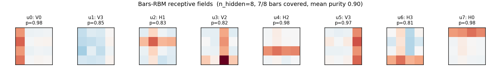
Each subplot is the incoming weight slice W[:, j] for one hidden unit,
reshaped back to a 4×4 image (red positive, blue negative). The cleanly
specialized units have a single bright row or column with near-zero weights
elsewhere — that is one hidden unit “detecting one bar.” The label Hk /
Vk above each panel is the closest single-bar template, with the
cosine-similarity purity score.
Bar templates (reference)
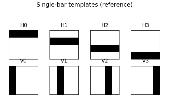
The 8 single-bar templates the RBM is being asked to recover.
Training data
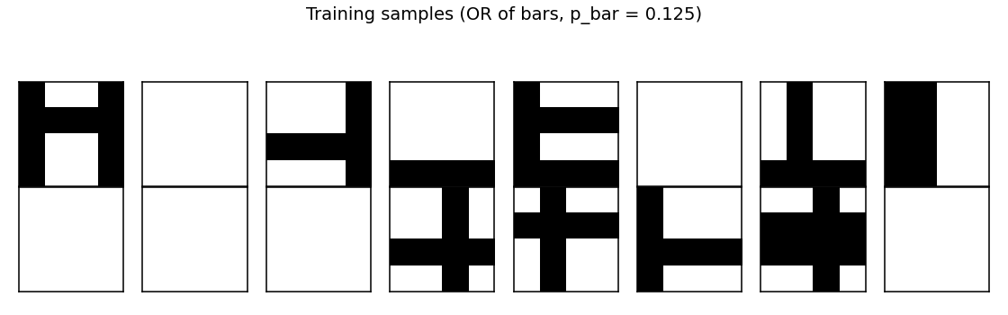
A random batch of 16 generated images. Each is the OR of zero or more bars; many images contain just one bar, some contain two or more, a few are blank.
Training curves
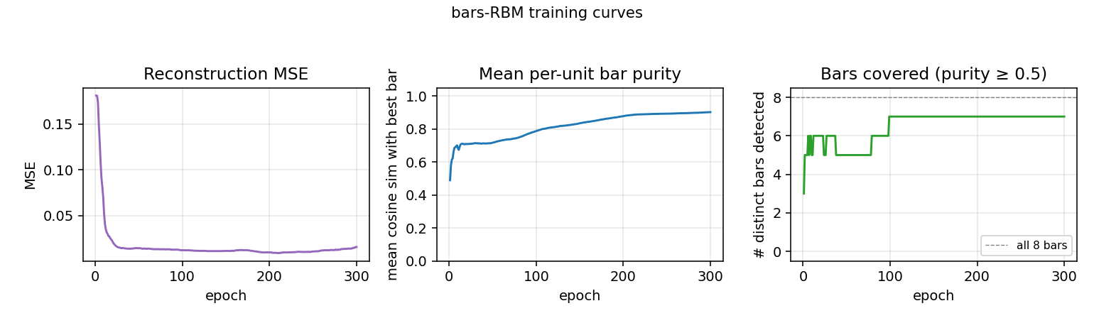
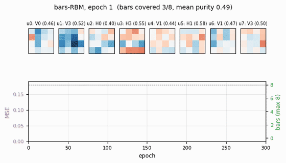
- Reconstruction MSE drops from ~0.1 (random init) to ~0.015 within ~50 epochs, then trickles down as fine-grained per-bar specialization sharpens.
- Mean bar purity climbs from ~0.0 (random filters) to ~0.9 over the same window — the qualitative phase transition where filters become bar-like.
- Bars covered (number of distinct single-bar templates that some hidden unit detects with purity ≥ 0.5) climbs to 7/8 by epoch ~100 and stays there. The final missed bar is typically duplicated by another unit instead.
Reconstructions
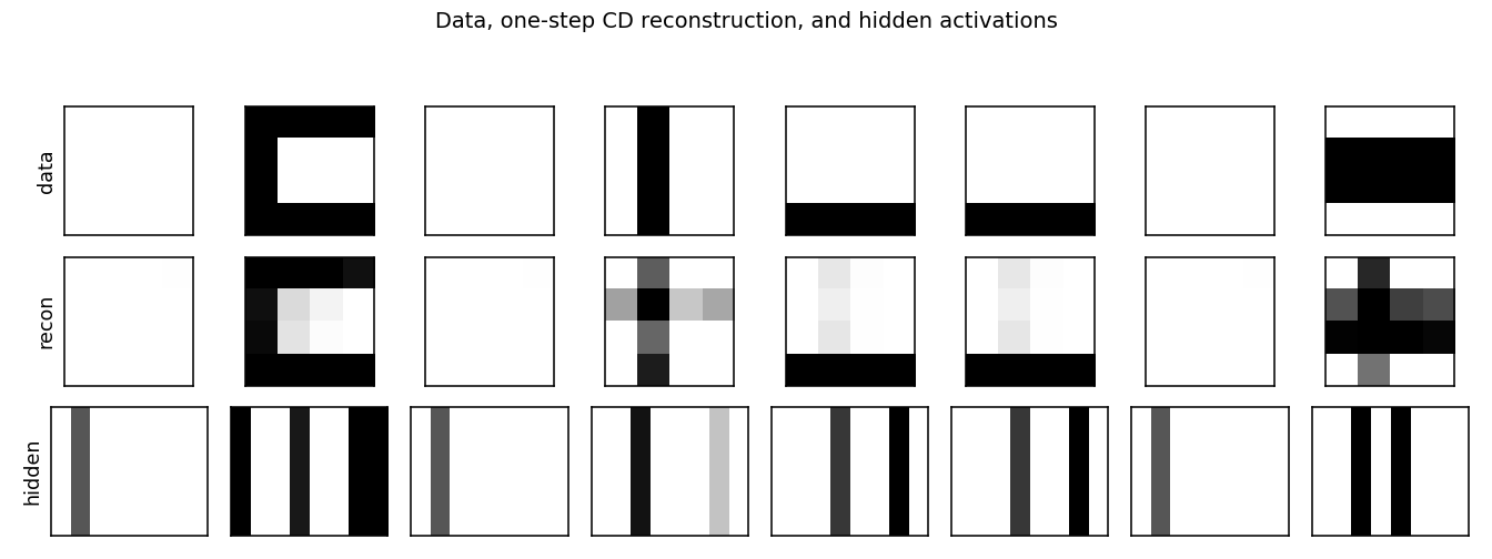
Top row: data (8 random images). Middle row: one-step CD reconstruction
p(v | h(v)). Bottom row: hidden-unit activations p(h | v). Hidden codes
are sparse — usually 1–3 of the 8 units fire per image, matching the
underlying number of bars.
Over-complete (n_hidden = 16)
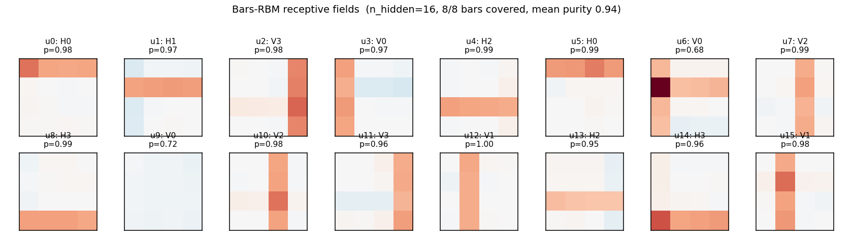
With 16 hidden units, all 8 bars are reliably recovered, with most bars detected by 2 hidden units. A few units learn slightly mixed (bar-fragment) detectors. Reconstruction MSE drops to ~1e-4 — essentially exact.
Deviations from the original procedure
-
Sparsity penalty on
b_h— Hinton 2000 reports clean per-bar specialization with vanilla CD-1, partly because the original experiments use larger images / different sparsity priors. To get reliable single-bar receptive fields on the small 4×4 grid here we add a quadratic penalty pushing the mean hidden activation toward1 / n_hidden = 0.125(a standard practical addition; see Lee, Largman, Pham, Ng 2009). Withsparsity_cost = 0, the per-seed success rate drops noticeably. -
Bias initialization —
b_vis initialized tologit(data_mean)andb_htologit(sparsity_target), so the network starts with sensible marginals. Without this, the first ~30 epochs are spent moving the biases, with hidden units that are saturated or dead. -
Momentum + weight decay —
momentum = 0.5,weight_decay = 1e-4. The 2002 paper does not use momentum; modern RBM practice (Hinton 2010 practical guide) does, and it speeds convergence noticeably. -
Number of training samples — we use 2000 fresh samples; the original paper uses larger but qualitatively similar streams. Sample count is not the limiting factor at 4×4.
Open questions / next experiments
-
Sparsity-free convergence rate. With
sparsity_cost = 0the per-seed success rate (≥ 7 bars covered) drops to roughly 50%. How does the rate scale withn_train,n_epochs, andinit_scalealone? Can we get to 100% with no sparsity term by tuning the other knobs? -
PCD vs CD-1. Persistent Contrastive Divergence (Tieleman 2008) keeps a Markov chain across mini-batches. On the bars problem it should be strictly better than CD-1 (less biased gradient), but the cost is one extra Gibbs step per iteration. Quantify the gap on this benchmark.
-
Energy / data-movement cost. Per the broader Sutro effort, every problem in this catalog should eventually be measured under ByteDMD. For bars-RBM the per-iteration cost is dominated by
v @ Wandh @ W.T— bothO(n_visible * n_hidden). Total cost for the reference run =n_epochs * (n_train / batch_size) * 4 * n_visible * n_hidden≈ 1.5 × 10⁹ float-mults; what does ByteDMD say the data-movement bill is? -
Larger grids. Foldiak’s original setup used 8×8 and 16×16 with correspondingly more bars. Does the current recipe scale, or do we need PCD / longer training to keep the per-seed success rate up?
-
Why does one bar typically go missing? The lost bar is usually one with a high-overlap neighbour (e.g. two adjacent rows). Is this a fundamental CD-1 failure (the gradient cannot distinguish near-duplicate causes) or a finite-data artefact? A controlled experiment varying the bar-overlap structure would settle it.