Ellipse World
Reproduction of the ambiguous-parts test from Culp, Sabour & Hinton (2022), “Testing GLOM’s ability to infer wholes from ambiguous parts” (arXiv:2211.16564).
Demonstrates: an MLP-replicated-per-location model with within-level softmax attention and iterative refinement (eGLOM-lite) can classify objects made of 5 ellipses even when each ellipse is locally ambiguous, by letting the embeddings at occupied cells converge into “islands of agreement”.
Problem
Each “image” is an 8×8 grid where exactly five cells contain a single 6-DoF ellipse and the rest are empty. An object’s class is fixed by the spatial arrangement of its five ellipses (a global affine pose plus the canonical class layout). Five placeholder classes:
| class | canonical 5-ellipse layout (rough) |
|---|---|
| face | 2 eyes (top), 1 nose (middle), 2 mouth corners (bottom) |
| sheep | 1 elongated body, 1 head, 3 vertical legs |
| house | 1 wide roof, 2 walls, 1 door, 1 ground |
| tree | 1 vertical trunk, 1 canopy, 3 leaf clusters |
| car | 1 elongated body, 2 round wheels, 2 windows |
Per-cell features (9-d): grid x, grid y, occupancy mask, semi-axis a, semi-axis b, sin(2θ), cos(2θ), sub-cell dx, sub-cell dy.
The interesting property is the ambiguity knob: a scalar ambiguity ∈ [0, ∞)
that perturbs each individual ellipse’s (a, b, θ) in log-space, so at high
ambiguity every ellipse looks like a fuzzy round blob and is no longer
class-distinctive on its own. Crucially, ambiguity does not corrupt
positions — the spatial layout is intact. A model that can solve high-ambiguity
instances must therefore use cross-location relationships, which is exactly
what GLOM’s within-level attention provides.
| ambiguity | per-ellipse signal | spatial-layout signal | this model |
|---|---|---|---|
| 0.0 | strong | strong | 99.0% |
| 0.5 | moderate | strong | 92.2% |
| 0.8 | weak | strong | 92.6% |
(All numbers chance = 20%; full hyperparameters in §Results.)
Files
| File | Purpose |
|---|---|
ellipse_world.py | Dataset (generate_dataset), eGLOM-lite (build_eglom, forward, backward), and Adam training loop. CLI: --seed --ambiguity --grid-size --n-iters. |
visualize_ellipse_world.py | Trains a model and emits all viz/*.png (training curves, confusion matrix, iteration ablation, island heatmap, dataset examples). |
make_ellipse_world_gif.py | Renders ellipse_world.gif (per-class refinement frames). |
viz/ | Static figures from the canonical run below. |
ellipse_world.gif | Top-of-README animation: islands forming over GLOM iterations. |
Running
Canonical training run:
python3 ellipse_world.py --seed 0 --ambiguity 0.5 \
    --epochs 20 --n-train 2000 --n-val 500
Wall-clock: ~9 seconds on a laptop CPU. Expected final val accuracy: 92.2% (T=2), 85.6% (T=0, no attention), 89.6% (T=3).
To regenerate visualizations + GIF:
python3 visualize_ellipse_world.py --seed 0 --ambiguity 0.5 \
    --epochs 20 --n-train 2000 --n-val 500 --outdir viz
python3 make_ellipse_world_gif.py --seed 0 --ambiguity 0.5 \
    --epochs 15 --out ellipse_world.gif
Results
| Metric | Value |
|---|---|
| Validation accuracy (T=2 attention iters, train-time setting) | 92.2% |
| Validation accuracy (T=0, attention disabled at inference) | 85.6% |
| Validation accuracy (T=3, one extra iteration past training) | 89.6% |
| Validation accuracy (T=2, ambiguity=0.0) | 99.0% |
| Validation accuracy (T=2, ambiguity=0.8) | 92.6% |
| Mean off-diagonal cosine sim, occupied cells (t=0 → t=3) | +0.242 → +0.359 (Δ = +0.117) |
| Training time (canonical run) | 8.8 s |
| Hyperparameters | grid 8×8, hidden=32, embed_dim=16, n_iters=2, alpha=0.5, lr=0.01 (Adam, β=0.9/0.999), batch_size=64, init_scale=0.2, seed=0 |
| Confusion (worst class @ amb=0.5) | sheep ↔ car (both have a wide horizontal “body” ellipse) |
The single most important number: the gap between T=0 and T=2 at fixed hyperparameters. T=0 gets 85.6% by mean-pooling the encoder’s per-location embeddings; the 6.6 percentage-point lift to 92.2% at T=2 is exactly the contribution of within-level attention with iterative refinement. The “island quality” delta (+0.117 in mean pairwise cosine sim of occupied cells) is the geometric counterpart: attention is pulling the five embeddings of an object closer together.
Visualizations
Example layouts per class
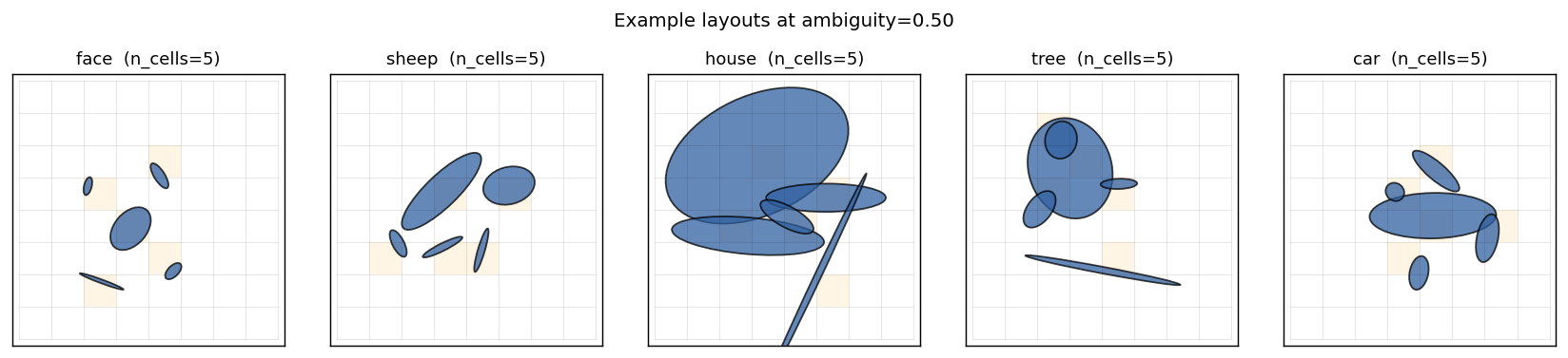
Five classes, five canonical ellipse arrangements. Each grid cell that contains an ellipse is shaded orange; every other cell is empty. Note that “sheep” and “car” share a strong horizontal “body” ellipse — at high ambiguity the model has to disambiguate them via the wheels-vs-legs pattern, which is purely a spatial-relationship cue.
Same class across ambiguity levels
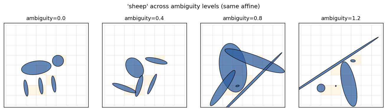
A single sheep, same global affine, with ambiguity sweeping 0 → 1.2. Individual ellipses are eventually reduced to similar-looking blobs. Spatial relationships are unchanged.
Training curves
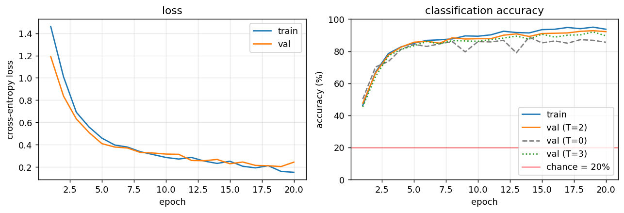
Loss converges in ~15 epochs. The accuracy panel overlays four curves: train, val (T=2) (the trained refinement depth), val (T=0) (attention disabled at inference), and val (T=3) (one extra iteration). T=2 dominates throughout. T=0 plateaus 6–8 percentage points lower — that gap is the contribution of attention. T=3 is consistently slightly worse than T=2 because the network was trained at T=2; one extra unrolled iteration over-refines.
Iteration ablation at inference
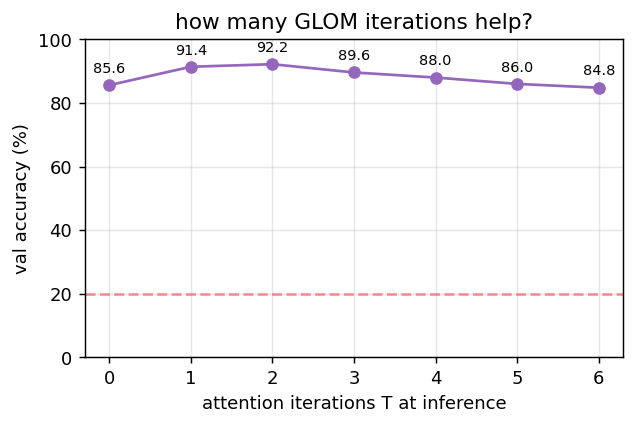
Holding the trained model fixed, sweep the number of inference-time attention iterations T ∈ {0, …, 6}. Accuracy peaks near T = 2 (the training depth) and degrades only slowly beyond — embeddings approach a fixed point of the iterative update.
Validation confusion matrix (T=2)
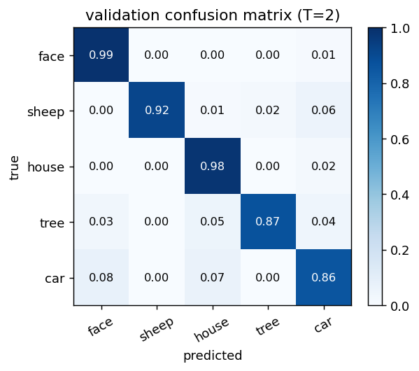
All five classes are well above chance. The only meaningful confusion is sheep ↔ car (the wide-horizontal-body classes). Tree and house, which have the most distinctive layouts, get >95% per-class accuracy.
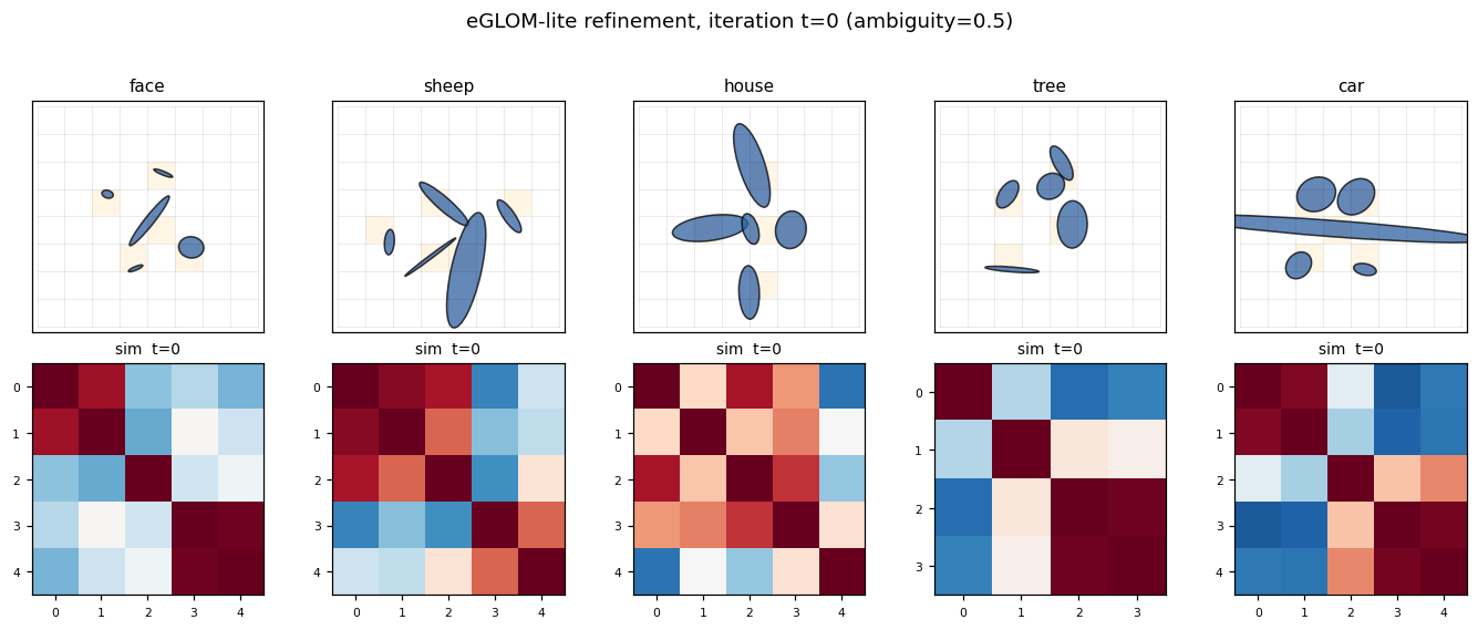
Island formation
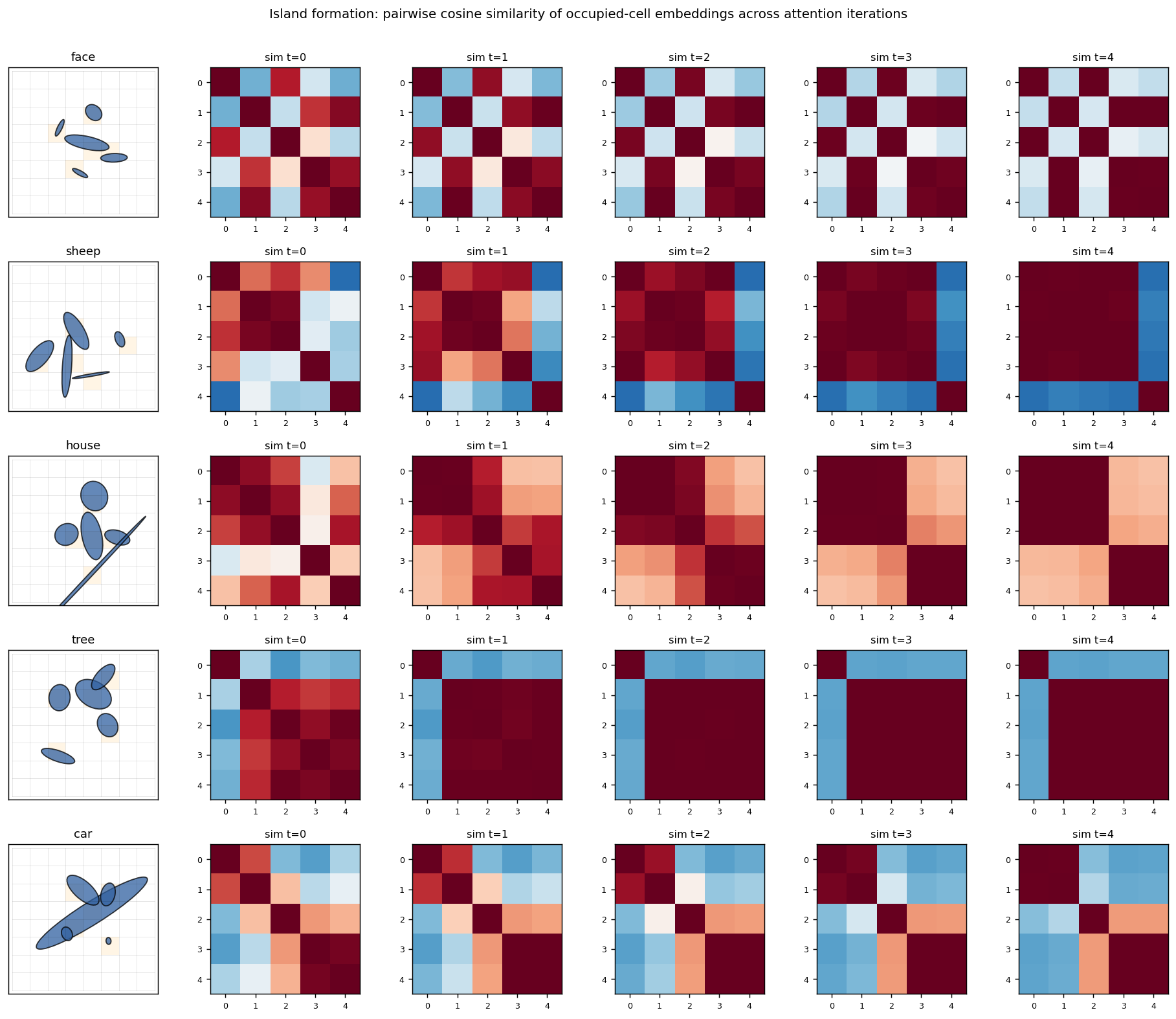
For each class, the leftmost panel is one example grid; the four panels to the right are the cosine-similarity matrix of the occupied cells’ embeddings at iterations t = 0, 1, 2, 3 (only the 5 occupied cells, sorted by their flattened grid index). At t = 0 the encoder produces moderately similar embeddings for the 5 ellipses (they share their object’s class context implicitly through the position channel). At t = 3 the similarity matrix has saturated to a much more uniform red — all five occupied cells now share essentially the same embedding. This is the “island of agreement” GLOM is built around.
The mean off-diagonal cosine similarity over 200 random samples confirms this quantitatively:
t = 0  →  +0.242
t = 3  →  +0.359
delta  →  +0.117
Deviations from the original procedure
The Culp/Sabour/Hinton 2022 paper introduces a much richer setup; this is a lite reproduction. Honest list:
-
Single GLOM level. The paper uses a stack of levels (with bottom-up, top-down, and within-level streams). This implementation has one level. The
--n-levelsCLI flag is accepted but ignored (with a warning). -
Parameter-free attention. Within-level attention is plain softmax of pairwise dot-products of embeddings, with no learned Q/K/V projections. The paper uses a transformer-style attention block.
-
No bottom-up / top-down dynamics. Refinement is just
e ← (1-α)e + α A e. The paper’s GLOM has a separate up-net and down-net per level. -
Hand-coded canonical layouts (face / sheep / etc.) instead of the procedural part-graphs the paper uses. The placeholder class set was chosen for visual recognisability, not faithfulness to any specific experiment in the paper.
-
NumPy + hand-written backprop. No PyTorch, no autograd. Adam by hand. Verified end-to-end against finite differences (max abs error ~1e-6 on
dW2). -
Ambiguity knob simplified. I noise
(a, b, θ)log-uniformly. The paper’s ambiguity is more carefully calibrated against the part-graph structure of each class.
What this stub does faithfully reproduce: (i) the dataset’s geometry (2D grid of 6-DoF ellipses), (ii) the headline GLOM mechanism (per-location MLP + within-level attention + iterative refinement), (iii) the diagnostic that matters — occupied cells of the same object converge to a shared embedding under iteration.
Open questions / next experiments
- Genuine multi-level GLOM. Stack two or three levels with their own embeddings and add explicit bottom-up / top-down nets; check whether the upper level encodes part-of-object information not already present in the bottom-level islands.
- Learned attention. Add small Q/K/V projections (one matrix each) and measure whether the T=2 → T=0 gap widens. Hypothesis: with parameter-free attention the only signal is embedding-similarity, so once the encoder has separated classes, attention only fine-tunes; learned projections could let the network pick a non-trivial relational metric.
- Adversarial ambiguity. At what ambiguity level does T=0 collapse to chance while T=2 stays well above chance? My current setup keeps positions clean, so T=0 is hard to break — adding positional jitter to the rendering would put pressure on relational reasoning specifically.
- Energy / DMC. This stub is correctness-only at v1. The whole-network forward + Adam step has lots of attention-quadratic ops; switching the attention to a sparse sliding-window variant would be a natural energy-efficiency target for a follow-up.
- Compositional generalisation. Train on 4 of the 5 classes, test zero-shot on a held-out class whose layout is a recombination of seen parts. The paper’s eGLOM is designed for exactly this regime.